I’ve been on annual leave for a few weeks. I’ve managed to catch up on all the challenges but haven’t blogged a solution for a while. It’s been a real struggle to get back into things to be honest – back to work, back to school, back to football clubs for my kids, and I’m wondering where I found the time before 😦
Trying to think about when/if I was going to get this blog out has caused me a bit of stress, which I don’t need, and so I need to change my mindset a bit…try to relax a bit … if I don’t manage to post a blog, just accept it and move on. I’ve also got to try to reduce the time it takes me to blog. I’m a ‘detail’ person, so often end up documenting to such a low level, but for my own sanity, I’m going to have to make an effort to be a bit briefer. I can’t guarantee I’ll stick to this though.. will just have to see how things pan out.
Going forward, I’m going to try to focus on the points that I think are key to the challenge, or those I found a bit tricksy.
So onto this week’s challenge. Sean Miller returned as guest poster with a COVID-19 related distance challenge.
Note – I connected to the provided hyper extract file rather than the csv file.
The core points I’m going to discuss are
Identify counties within n miles
How to select a county without set actions
How to handle ‘All’ counties being selected
Colouring based on ‘percentile’ of hospital beds
How to only show county borders of counties within selected range
Identify counties within n miles
The number of miles is stored within an integer parameter, n miles, that is defaulted to 100.
A county to act as the ‘start point’ is stored in a set, Selected County, based on the County, State field.
The long/lat coordinates of this selected county need to be captured.
Selected County Lat
{FIXED : AVG(IF [Selected County] THEN [Latitude] END)}
Selected County Long
{FIXED : AVG(IF [Selected County] THEN [Longitude] END)}
By using a FIXED LoD calculation, the values are stored against every ‘row’ in the data set.
With these, the starting point can be determined
Selected County Start Point
MAKEPOINT([Selected County Lat],[Selected County Long])
The position of every other county – the ‘destination’ / end point – also needs to be determined
End Point
MAKEPOINT([Latitude],[Longitude])
With these, the distance between can be computed
Distance
DISTANCE([Selected County Start Point],[End Point],’miles’)
And the counties can then be restricted by
Within n miles
[Distance]<= [n miles]
which can be used as a filter and set to True.
How to select a county without set actions
This is managed via the set control feature; right click on the Selected County set and choose Show Set to display the list of counties with the option to select which ones are in or out of the set. Change the display of the control via the dropdown arrow (top right) to be Single value dropdown which automatically provides as ‘All’ option or the ability to select a single set only.
How to handle ‘All’ counties being selected
When ‘All’ is chosen via the Set Control selector, this has the effect of adding all the State, County values into the set, which means we don’t really have a starting state. So the n miles parameter is essentially redundant. But we need to make the Within n miles filter understand this.
We can manage this by first identifying how many values we have in the set
Count Selected States
{FIXED : COUNTD(IF [Selected County] THEN [County, State] END)}
There will either be 1 or if All is selected, then they’ll be 3000+, and we use the FIXED LoD, so the total is stored against all rows.
We can then update our Within n miles filter to consider this value
Within n miles
([Count Selected States]=1 AND [Distance]<= [n miles]) OR [Count Selected States] > 1
This now returns true if either one State, County is selected and the other records are within n miles OR all the states are selected (the count is > 1).
Colouring based on ‘percentile’ of hospital beds
This caused me a little bit of headscratching. I assumed ‘percentile’ would be based on a percentage of the total num_staffed_beds (note I simply renamed this field to Hospital Beds), associated to the state,counties being displayed (ie within n miles). But after building the calculation I thought, and adding it to colour and choosing the Green-Gold colour range, I didn’t get the same spread as shown in the solution.
I messaged Sean to question whether I’d made the right assumption, but while waiting for a response, I did an online search for “Tableau Percentile Rank”, and quickly spotted that a Table Calculation exists. As you can guess, I don’t use this particular calculation very much at all 🙂
So to colour, add Hospital Beds , and simply add a Percentile table calculation
How to only show county borders of counties within selected range
When working with Maps, you can use the options within the Map Layers menu to select which features of the map should be displayed. One of these options is State/Province Borders, which you might think is what is needed.
However, this will show all the state borders, which is evident if you zoom out a bit, including those for states that don’t have counties within n miles.
This isn’t the requirement – we only want to show the borders of the states which have counties within the desired range. So instead, we don’t want to show any State/Province Borders via the Map Layers. And we’ll utilise a dual axis instead, by first identifying the states that are within n miles
States within n miles
If [Within n miles] THEN [State] END
Duplicate the Latitude (generated) field on the Rows, remove all the fields on that mark, and then add the States within n miles to the Detail shelf. Set the colour of this mark to white, and swap the Latitude (generated) fields if needed, so the States are on the top, as below.
Then make dual axis 🙂
And that’s the key points that I hope will help you solve this challenge. My published version is here, which is available to be downloaded. If there’s anything I haven’t covered that you’re not sure about, feel free to contact me.
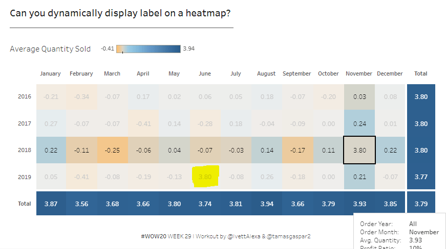
For this week’s challenge, Ann asked we recreated a scatter plot that ‘on click’ became a connected scatter plot and also displayed an ‘insights’ box to the user.
Building out the data
The scatter plot is to show Profit Ratio by Quantity, so first up we need
Profit Ratio
SUM([Profit])/SUM([Sales])
formatted to percentage with 0 dp.
A mark is shown on the scatter plot per Category and Month/Year. When working with dates like this, I often prefer to created a dedicated field to use as an ‘exact date’ which I can then format. So I built
Month Year
DATE(DATETRUNC(‘month’,[Order Date]))
and formatted it to the March 2001 format (ie mmmm yyyy).
We’re also going to need a set based on the Category field, as that is going to drive the interactivity to help us connect the dots ‘on click’. So right click on Category and Create Set and just tick one of the categories displayed for now.
Selected Category
Let’s build these out into a table as follows
Order Date to Filter, filtered by years 2018 & 2019
Category, Selected Category & Month Year (exact date , discrete) onto Rows
Measure Names to Text and Filter to Quantity & Profit Ratio
Right click on Selected Category and select Show Set to display a selection control to easily allow the set values to be changed
To help drive the interactivity, we’re going to need to store the value of the Profit Ratio for the Selected Category in the set.
Selected PR
IF ATTR([Selected Category]) THEN [Profit Ratio] END
Format this to percentage 0 dp too, and add this to the table – it will only display the profit ratio against the rows associated to the category in the set
At this point, we’ve got what we need to build out the scatter plot, but I’m going to continue to create the fields needed for the ‘Insights’ piece.
These are looking for the months that contained the Max & Min values for the Profit Ratio and Quantity. I’m going to tackle this with Table Calcs.
Max PR per Category
WINDOW_MAX([Profit Ratio])
Adding this to the table, and setting the table calculation to compute by Month Year only, gives us the Max Profit Ratio for each Category
We need 3 more fields like this :
Max Qty per Category
WINDOW_MAX(SUM([Quantity]))
Min PR per Category
WINDOW_MIN([Profit Ratio])
Min Qty per Category
WINDOW_MIN(SUM([Quantity]))
Add all these to the table, setting the table calc in the same way as described above.
Now we know what the min & max values are, we need to know the month when these occurred.
Max PR Month
WINDOW_MAX(IF ATTR([Selected Category]) AND [Profit Ratio] = [Max PR per Category] THEN MIN([Month Year]) END)
Format this to March 2001 format.
If the category is that selected, and the profit ratio matches the maximum value, then retrieve the Month Year value, and duplicate that value across all the rows (this is what the outer WINDOW_MAX does).
Add this to the table in the Rows, and adjust the table calc settings for both the nested calculations to compute by Month Year only. The month for the selected category which had the highest profit ratio will be displayed against all rows for that category, and null for all other rows.
Again we need similar fields for the other months
Max Qty Month
WINDOW_MAX(IF ATTR([Selected Category]) AND SUM([Quantity]) = [Max Qty per Category] THEN MIN([Month Year]) END)
Min PR Month
WINDOW_MAX(IF ATTR([Selected Category]) AND [Profit Ratio] = [Min PR per Category] THEN MIN([Month Year]) END)
Min Qty Month
WINDOW_MAX(IF ATTR([Selected Category]) AND SUM([Quantity]) = [Min Qty per Category] THEN MIN([Month Year]) END)
Format all these too, and add to the table with the appropriate table calc settings applied.
If you now change the value in the the Selected Category set, you should see the table update.
Building the Scatter Plot
On a new sheet, build out the basic scatter plot by
Order Date to Filter, filtered by years 2018 & 2019
Profit Ratio to Rows
Quantity to Columns
Category to Colour and adjust accordingly
Month Year exact date, continuous to Detail
Change Shape to filled circle
Adjust the Tooltip to suit
Change the axis titles to be capitalised
Change the sheet title
Remove all row/column borders & gridlines. Leave the zero lines and set the axis rulers to be a sold grey line
Add Selected PR to Rows, and change the mark type of that card to line, and add Month Year to path. In the image below, I still have Furniture selected in my set.
Add Month Year to the Label shelf too and format so the text is smaller and coloured to match mark colour
Make the chart dual axis, synchronise the axis and remove the Measure Names from the colour shelf of each mark. Hide the Selected PR axis.
If you now change the selected set value, you can see how the other categories ‘join up’.
Building the Insights Box
Take a duplicate of the data table built originally, and add Selected Category to Filter. If you’ve still got an entry in your set, this should reduce the rows to just those records for that Category.
Remove the fields Profit Ratio, Quantity, Selected PR from the Measure Values section, and remove Selected Category from Rows.
Create a new field
Index = Size
INDEX()=SIZE()
and add this to the Filter shelf, setting the value to true.
The INDEX() function will number each row, the SIZE() function will number each row based on the total number of rows displayed (ie all rows will display the same number), so INDEX()=SIZE() will return true for the last row only
Now we’ve only got 1 row displayed, we’ve got the info we need to build the data in the Insights box by
Move Month Year to Detail
Category to Colour
Move Max PR Month, Max Qty Month, Min PR Month, Min Qty Month to Text
Move Max PR per Category, Max Qty per Category, Min PR Per Category, Min Qty per Category to Text
This will probably show duplicate instances of the values. This is because we didn’t fix the table calculation setting of the Index=Size field. Edit that to compute by Month Year
and then re-edit the Index=Size filter to just be true again, and expand the display so you can see all the values.
Now you can easily format the Text to the required display
I used this site to get the bullet point image from
Building the dashboard & interactivity
Add the scatter plot to the dashboard, and remove the legends that automatically get added.
Float the Insights sheet and position bottom right, remove the title. fit entire view, and also remove the colour legend which will have been added.
Add a dashboard Set Action to assign values to the Selected Category set and remove all values when the selection is cleared
Additionally, add a highlight action that highlights the Category field only (this keeps the lines highlighted on selection of a single mark).
Now practice clicking on and off marks on the scatter plot and you should see your lines & insights box being added and removed.
Finally add the title and header line by adding a vertical container at the top above the scatter plot.
Add a text box for the title, and underneath add a blank object.
Set the padding of the blank object to 0 and the background to black. Then edit the height to 4, and adjust the height of the container if it’s now too large.
Make adjustments to the position of the floating insights box if need be so it isn’t overlapping any axis.
This viz is essentially equivalent to a small multiple display where the charts for a specific dimension (in this case State) get displayed across numerous rows and columns. The difference here, is the row and column for the State to be displayed in, is specifically defined, rather than just sequentially based on how the data is being sorted.
Luke very kindly provided the logic to determine the rows and columns.
Building out the data
Once again, I’m going to start by putting all my data into a table so I can check my calculations, especially since this challenge does involve table calculations (there’s a hint on the Latest Challenges page)
Data Source Filter
Although not explicitly mentioned in the requirements, the information we need to present is based on the dates from 1st March 2020 to 31st July 2020. I messaged Luke to check this, before I then realised it was stated in the title of the viz – doh!
To make things easier, I therefore added a data source filter to remove all the other dates, setting the Report Date to range from 01 March 2020 to 31 July 2020 (right click on the data source -> add data source filter
I then added the basic fields I needed to a table
Province State Name to Rows
Report Date discrete, exact date (blue pill) to Rows, custom formatted to mmmm, dd
People Positive New Cases to Text
I excluded the fields where Province State Name = Null
We need to calculate the 7 day rolling average per Province State Name which we can do by using the UI to create a Moving Average quick table calculation against the People PositiveNew Cases pill, and then editing to compute over the previous 6 records (+ the current record makes 7 days). But I want to be able to reference this field, so I’m going to ‘bake it’ into the data model by creating a specific calculated field
7 day moving Avg
WINDOW_AVG(SUM([People Positive New Cases Count]), -6, 0)
Add this into the table, and edit the table calculation to compute by Report Date only and set the Null if not enough values checkbox
Do a basic sense check that the averages are correct by summing up 7 sequential rows and working out the average by dividing by 7.
So it looks like we’ve got the core measure to be plotted, but we’re going to need some additional fields in the presentation.
Again it’s not explicitly stated in the requirements, but it is in the title, that the values plotted need to be normalised. This is to ensure the data for each state is visible; if a state with a relatively low number of cases is positioned in the same row as one with a very high number of cases, it will be hard to see the data for the state with the low cases, because while the axis can be set to be independent, this will only work against a row and not an individual instance of a chart.
To normalise, we need to understand the maximum 7 day rolling average for each state.
Max Avg Per State
WINDOW_MAX([7 day moving Avg])
Add this to the table, setting both the nested table calcs to compute by Report Date.
In normalising, what we’re essentially going to do is determine the 7 day moving Avg as a proportion of the Max Avg Per State, so every value to plot will be on a range of 0-1.
Normalised Value
[7 day moving Avg]/[Max Avg Per State]
Format this to 2 dp, and add to chart, remembering to check the table calcs continue to compute by Report Date only.
Above you can see the max value for Alabama occurred on 19th July, so the Normalised Value to plot is 1
In the chart displayed, each State is titled by the name of the State. In a small multiple grid of rows & columns, we can’t use a dimension field for this, as it won’t appear where we want it. Instead we’re going to achieve this using dual axis, and plotting a mark at the centre point. For this we need to determine the centre date
This looks a bit complex, so I’ll break it down. What we’re doing is finding the number of days between the minimum date in the data set and the maximum date in the data set. This is
We’re then halving this value ( /2) and rounding it down to the nearest whole number (FLOOR).
We then add this number of whole days to the minimum date in the data set (DATEADD), to get our central date – 16 May 2020.
Now we need a point where we can plot a mark against that date. It needs to be above the maximum value in the main chart (which is 1). After a bit of trial and error, I decided 1.75 worked
Plot State
IF [Report Date] = [Centre Date] THEN 1.75 END
Finally we need to create our Rows and Columns fields which provides the co-ordinates to plot each state. The calculations for these were just lifted straight out of the requirements – thanks Luke!
Building the Viz
Start by adding the Rows and Columns fields to their respective shelf. Set them to be discrete dimensions (blue pills). You should immediately see a ‘map’ type layout of the US States.
Exclude the Null Rows value.
Now add Report Date as a continuous exact date (green pill) to Columns and Normalised Value to Rows, remembering to set the table calc to compute by Report Date only for all nested calculations. Change the mark type to Area.
Add 7 day moving Avg to Label and set the label to display the max value only and adjust the font size – I ended up at 7pt. Then add Province State Name & People Positive New Cases Count to Tooltip. Format the tooltip to match.
Remove all column/row lines and grid lines, zero lines etc.
There is a requirement to ‘add a line underneath each of the area trends’.
For this I added a 0 constant reference line formatted to be a solid black line.
But you’ll notice that for the charts that sit directly side by side, the line seems to be continuous, but I want to break it up. I re-added the column divider line to be a thick white line to get the desired effect.
Right, now lets get the State label added.
Add Plot State to Rows before Normalised Value and change the aggregation from SUM to MIN.
Change the Mark Type to Text and move the Province State Name field from Tooltip to the Text shelf. Adjust the text label to remove any other fields that are displaying, and resize the font – again I used 7. Clear the Tooltip for the this mark, so nothing displays on hover.
Make the chart dual axis and synchronise axis. Remove the Measure Names pill from the Colour shelf on both marks cards which will have automatically been added.
And now all you need to do is remove all the headers (uncheck Show Header) against Rows, Columns, Report Date & Plot Value, then right click on the >8k nulls label at the bottom right and select Hide Indicator.
You’re all done – you just need to add to a dashboard now. My published version is here.
I really enjoyed this challenge – a nice mix of calculations & format complexity but not overly cumbersome, which meant this blog didn’t take so many hours to write this week 🙂
The #WOW2020 week 31 challenge was combined with a #PreppinData challenge and launched at a virtual live event. I was fortunate enough to be able to join this event for the first hour and had the pleasure of meeting up with some #WOW regulars Sean Miller, Kyle Yetter & Tim Beard, along with #WOW challenge setter Lorna Brown, and #PreppinData setters, Jenny Martin and Tom Prowse. I was gutted I couldn’t stay on for the whole session, but work commitments got in the way – bah!
I did complete the #PreppinData challenge first, and the last time the team ran a combined event, I did blog on how I built both challenges, but I’m struggling for time, and the #WOW has got a fair bit going on, so I’m afraid the Prep challenge won’t make the cut this time – sorry #Preppers!
So onto the #WOW challenge. Part of this challenge was to utilise the new Relationships feature in 2020.2, so you need to be on this version to follow along.
Creating the data source
If you’d completed the #PreppinData challenge, you could use your own outputs as the inputs for #WOW challenge. I did that initially, but as I was building I had a few minor discrepancies from the solution, so chose to replace my data sources with the hyper files that are referenced in the Prep challenge, these being
Host Countries – 1 row per Olympic Host City (and Country) per Year since 1896 to 2016
Country Medals – 1 row per Country attending the Olympics per Year, summarising the number of Bronze, Silver and Gold medals won by that country.
Medalists – For every Country, for every Year, there is 1 row per Athlete who won a Medal including the type of Medal (Bronze, Silver, Gold).
In Tableau Desktop, connect to the Host Countries hyper file and drag the ‘table’ named Extract into the data source pane. If you right click on the table, you can the rename it – I chose Host.
Then Add a connection to the Country Medals hyper file, and again drag the ‘table’ named Extract into the data source pane so it connects to the Host table. Set the relationship to be on Year. I renamed the ‘table’ again to be Medals.
Now add another connection to the Medalists hyper file, and drag the ‘table’ named Extract to connect to the Medals table, this time setting the relationship both on Country and Year. I renamed the ‘table’ again to be Medalists.
Building the Bump Chart
As with many challenges, if I can, I build the data I need into a table to start with, so I can check my calculations, so lets get the basics
Note – depending on the order you connected your tables in the data source, some field names that exist in multiple tables will be suffixed with fieldname (Extract x). I won’t refer to the Extract part, but will reference fields I use in this blog by prefixing with the table name instead.
Drag out Host.Year, Host.Host Country, Medals.Country to Rows. Lets show the number of medals of each type each country won, so we can use this to sense check some calculations later : put Medals.Gold, Medals.Silver, Medals.Bronze into the table
The bump chart we need to build is ranked based on the score of each country which in turn is determined by giving 3 points for each gold medal, 2 for a silver and 1 for a bronze, so we need a calculated field
We need to rank this score, and I’m going to have a calculated field to store this explicitly
Rank Score
RANK_UNIQUE([Score])
Add these 2 fields to the table, and adjust the table calculation of Rank Score so all fields except Year are ticked
Now we could start building out the bump chart now, and I did when I was creating this and would then flit back and forth between doing something on the chart and checking new calcs. However, to keep the blog a bit easier, we’ll continue building out the table.
So first up, we need another rank field. When building out the bump chart initially, I was doing all sorts of things to show the Top 10 only, but whatever I did, I couldn’t stop the lines from joining up between countries when they didn’t exist in consecutive years eg Greece is 1st in 1896, but doesn’t appear in the Top 10 again until 1904. As 1900 was missed, the lines shouldn’t join, but mine were. I was faffing over this for some time, so eventually caved and checked out Lorna’s solution. She’d resolved this simply with
Top 10 Rank Only
IF [Rank Score] < 11 THEN [Rank Score] ELSE NULL END
ie only show the rank if its in the Top 10. Simples really!
Add this onto the table and check the table calculation setting is as previously.
So for the bones of the bump chart we have the two fields we’re going to plot against – Year and Top 10 Rank Only, but before we do that, let’s get the fields we need that are displayed on the tooltip.
# Countries Per Year
{FIXED [Year] : COUNT([Medals])}
This will give us the number of countries that participated in each year. The COUNT([Medals]) comes from dragging the Medals(Count) that is automatically generated as part of the Medals table into the calculated field dialog- in the new Relationships model, this Count field against each table is essentially the equivalent of Number of Records.
A simple tally of the total number of medals won by each country.
Is Host?
[Host Country]=[Country (Extract2)]
where this is checking Host.Host Country against Medals.Country and returns true if they match.
Hosted | Participated
IF [Is Host?] THEN ‘hosted’ ELSE ‘participated’ END
The text on the tooltip differs slightly dependent on whether the country hosted or not.
COLOUR: Country
IF [Is Host?] THEN [Host Country] END
The stars on the bump chart need to be coloured based on country, but we don’t want the circles coloured too, so this field is necessary.
Let’s get all these into our table… you’ll notice (or you may not), but adding some of these fields causes the Rank Score & Top 10 Rank Only to change, so readjust the tableau calculation so only Year remains unchecked.
Now we have everything to build the core bump chart.
Add Host.Year to Columns, Medals.Country to Detail and then add Top 10 Rank Only on Rows. Change the Mark Type to a Line, and verify the table calculation on the Top 10 Rank Only is set to compute by Country only.
Edit the Top 10 Rank Only axis and set the scale to be reversed
Change the Colour to grey and make the Size smaller.
Thenadd another instance of Top 10 Rank Only to site alongside the existing one on the Rows.(I tend to click on the existing pill, hold down ctrl and then drag – this will create a duplicate instance and will retain the table calculation settings).
Now make the chart dual axis & synchronise the axis.
Change the mark type of the second axis to be a shape, and add Is Host? to the Shape shelf. Adjust so that false is a filled circle and true is a filled star.
Also add Is Host? to the Size shelf on this marks card, and adjust the sizes so true is bigger than false.
At this point you will need to adjust the table calculation of the 2nd Top 10 Rank Only pill, to compute by both Country and Is Host?.
Add COLOUR: Country to the Colour shelf, and adjust the colours to use the Hue Circle palette. Set the NULL value to the same shade of grey as the line.
You’ll need to adjust the table calculation again of the 2nd Top 10 Rank By County pill, so only Year is unselected.
All the following fields need to be added to the Tooltip of the All marks card.
Score
# Countries Per Year
Hosted | Participated
Top 10 Rank Only (setting the table calc to compute by everything except Year)
# Medals
Adjust the Tooltip accordingly, then tidy up the formatting of the chart
Hide the Top 10 Rank Only axis
Rotate the labels of the Year
Hide the Year field label
Remove all row & column lines and gridlines/zero lines
Medals Viz in Tooltip
The Bump chart has 2 Viz in Tooltips, one showing the count of the different medals won and the other showing the top 10 athletes. Build the Medals chart by
Host.Year to Rows
Medals.Country to Rows
Medals.Bronze to Columns
Then drag the Medals.Silver pill to the bottom of the chart where the Bronze axis is, and when you see 2 green columns, drop the pill. This should have the effect of Measure Values automatically being added to Columns, and Measure Names being automatically added to Rows and the Filter shelf.
Then add Medals.Gold into the Measure Values pane
Reorgansie the pills in the Measure Values pane so they are listed Gold, Silver, Bronze
Add Measure Names to Colour and adjust accordingly
Show the mark Label
Now hide the Year and the Country columns, and the Value axis at the bottom. Remove all the formatting (the quickest way is to go to the bump chart sheet you should hopefully have formatted already, right click on the tab of the sheet at the bottom, and select Copy Formatting, then go back to the sheet you’re working on, and on the tab, right click & Paste Formatting
If this doesn’t clean everything up enough, just adjust formatting manually.
Finally, set the fit on this sheet to be Entire View. This will squash everything up, but when its referenced from the viz in tooltip, the view will be filtered to the Year and Country. Doing this will remove the ‘this view is too large’ message that may appear on the Viz in Tooltip.
Switch back to the Bump chart and add the sheet to the Tooltip by Insert -> Sheets -> <Select your sheet>. Adjust the maxwidth property to 500 and maxheight property to 100 to make the viz fit better
Top 10 Athletes Viz in Tooltip
Build the initial viz by
Host.Year to Rows
Medals.Country to Rows
Medalists.Athlete to Rows
Medalists,Medal to Columns and manually reorder the columns.
Medalists.Medalists(Count) to Columns
Medalists.Medal to Colour
To work out the Top 10, we need to first work out the score per medal
Medalist Score
CASE [Medal] WHEN ‘Gold’ THEN 3 WHEN ‘Silver’ THEN 2 WHEN ‘Bronze’ THEN 1 END
then calculate the total score per athlete per games, since an athlete can win more than one medal and appear in multiple games
We only want the Top 10 though, so add Athlete to the Filter shelf, and filter by the top 10 of Total Score per Athlete
At this point, things won’t look right, as the filter will be applying over all the data. To get this right, we now need to add the sheet to the Viz in Tooltip, so go back to the Bump chart, and on the tooltip add a reference to this sheet.
Adjust the width and explicitly filter by Host.Year, Medals.Country
If you now return to the Top 10 sheet, an additional filter will have been automatically added to the Filter shelf. Add this filter to context, so it will change to a grey pill.
Now return to the Bump chart and just test out that the chart is presenting correctly when hovering over various fields.
Now return to the Top 10 chart and tidy up all the formatting and hide various fields, and set to Entire View.
The bump chart should now be complete
Building the strip plot
The strip plot is showing a mark for each host with an indicator to show if they finished in the Top 10 or not. Additional information on the tooltip shows the host’s score and medals count. We’ll build this into a table first as below
We ultimately need to show 1 row per year, but the country level data is required to work out the rank. So we’re going to use some more table calculations.
We want to capture the host’s score and medals accrued against all the rows associated with each year.
Score for Host
WINDOW_MAX(IF ATTR([Is Host?]) THEN [Score] END)
Medals for Host
WINDOW_MAX(IF ATTR([Is Host?]) THEN [# Medals] END)
Add these to the table, setting the table calculation to compute over all fields except Year.
We also need to know if the host was in the top 10 or not
Is Host in Top 10?
WINDOW_MAX(IF ATTR([Is Host?]) AND [Rank Score]<=10 THEN 1 ELSE 0 END)
Add this onto the table, and again, sense check the table calculations (this one is nested) to ensure all are computing by all fields except Year
So we have all the bits of data we’ll need, we just need to reduce to 1 row per year.
Index = Size
INDEX() = SIZE()
Add this onto the Filter shelf, and set to true. Check the table calculation again to ensure all fields except Year are set. Recheck the filter is still only selecting true.
This should reduce the data, and just show the last row listed for each country.
For the strip plot, add
Host.Year to Columns
Medals.Country to Detail
Mark Type to Shape
Is Host in Top 10? to Size and to Shape. Adjust the table calcs and shape/size accordingly (you’ll need to reverse the size).
Host Country to Tooltip
Medals for Host to Tooltip (remember table calc)
Score for Host to Tooltip (remember table calc)
Index = Size to Filter set to true (again remember table calc)
Change colour to red
Adjust Tooltip accordingly
Finally adjust the formatting, and remove the header.
Top 10 Countries Viz in Tooltip
Add Host.Year, Host Country and Medals.Country to Rows and Score to Columns, then click the Sort button in the menu to sort the Country descending. Add Rank Score to Rows and change to be discrete (blue pill). Move it to sit in front of the Country field
We need to restrict the rows based on whether the Country in is the top 10 or it’s the host country
Is Host or Top 10?
ATTR([Is Host?]) OR [Rank Score]<=10
Add this onto the Filter shelf and set to true; once again make sure the table calc is computing by all fields other than Year (and double check its still set to true after adjusting). If you scroll to the bottom, you should see 11 rows for 2016, as the host, Brazil, finished 12th.
And now we need to colour the bars
COLOUR:Host
IF [Rank Score] > 10 THEN ‘Red’ ELSEIF ATTR([Is Host?]) THEN ‘Blue’ ELSE ‘Grey’ END
Add to the Colour shelf and adjust accordingly. Then add Score and # Medals to the Text shelf and format the label displayed. Finally hide some of the fields and format the chart to remove axis/gridlines etc.
Finally, set the fit to Entire View.
Go to the strip plot chart and add this sheet to the Tooltip, setting the filter to be on Year
And that should be all the components you need to build the dashboard.
For week 30, #WorkoutWednesday alumni Emma Whyte returned re-posting this challenge which was originally set in Week 41 of 2017 (see here). The idea behind this was to see how the challenge could be achieved using features that have been released since that challenge – in this case set actions.
I’ve been doing the #WorkoutWednesday challenges since they were first introduced, so I completed the original challenge, which is posted here.
Despite it being over 2 1/2 years ago, I had a strong recollection as to what was required to achieve this. So the challenge I set myself, was to recreate without looking at my own solution.
Building out the data
This is one of those challenges where we can build the data out into a table to check the functionality before building the actual viz. I always like to do this where possible, as I find it a good reference to make sure I’m getting the logic & the calculated fields I need right.
Start by adding State & City to Rows and add Sales & Profit via Measure Names on Columns .
As the challenge is to use Set Actions, then naturally, we’re going to need a Set. The Set we need is based on State with the idea being that when there is a State(s) in the set, then the City will display instead.
Selected State
Right click on State and Create -> Set. Select an option in the dialog, eg Alabama say
We will need to show the marks based on State or City depending on whether a State has been selected or not. We need a single field that we will use in the viz that displays the dimension we need to show
Display Value
IF [Selected State] THEN [City] ELSE [State] END
Add this onto the Rows and you’ll see how this is working
We can test the functionality of putting values into and out of the set without the need for the dashboard action at this point, by right-clicking on Selected State and selecting Show Set – the list of set values to select will display (a bit like a filter list).
We need a way to figure out what rows to show – how to identify whether there’s anything selected in the set.
Count States Selected
{FIXED : COUNTD(IF [Selected State] THEN [State] END)}
By being an LOD, this will set the count of the items in the set across all the rows in the data. Add to the sheet so you can see how this works
So we want to show information when either there isn’t anything in the set, or for the rows associated to the Selected States only
Records to Show
[Count States Selected] = 0 OR [Selected State]
Add this to Rows and test out… with no State in the set, all the rows are True
but with a State selected, only the rows associated to that State are True
But we seem to have too many marks showing when there’s nothing in the set….?
That’s fine.. just take City out of the view now, and if you deselect all States you should get the 48 rows we’re going to start with listed, and all are Records to Show = True. The Sales & Profit values will also now be aggregated to the appropriate level.
Building the Viz
Ensure your Selected States set is empty, and build out the scatter plot
Profit on Columns
Sales on Rows
Display Value on Detail & Label
Records to Show on Filter set to True
Mark Type = Shape set to x
Verify the functionality by clicking a State in the list, and the view should change to show the City.
We need to colour the marks based on Profit
-ve Profit?
SUM([Profit])<0
Add this to the Colour shelf and adjust colours accordingly.
Finally we need to look at how the title/subtitle changes based on which level we’re at.
Title
IF [Count States Selected] = 0 THEN ‘Sales vs. Profit by State’ ELSE ‘Sales vs. Profit for ‘ + [State] END
Subtitle
IF [Count States Selected] = 0 THEN ‘Select a state to drill down to city level’ ELSE ‘Double-click a city to drill up to state level’ END
Add these onto the Detail shelf, then they’ll be available to reference in the Title of the sheet.
And then adjust the Tooltip, and we’re pretty much ready to go.
Adding the Set Action
Create a dashboard and add the scatter plot sheet to it.
Add a dashboard action to Change Set Values which runs on the Select action, and assigns values to the Selected State. On clearing the selection, values are removed from the set.
And that should pretty much be it. My published version is here. I thoroughly enjoyed the ‘throwback’ to previous challenges, and would like to see this theme continue on occasion.
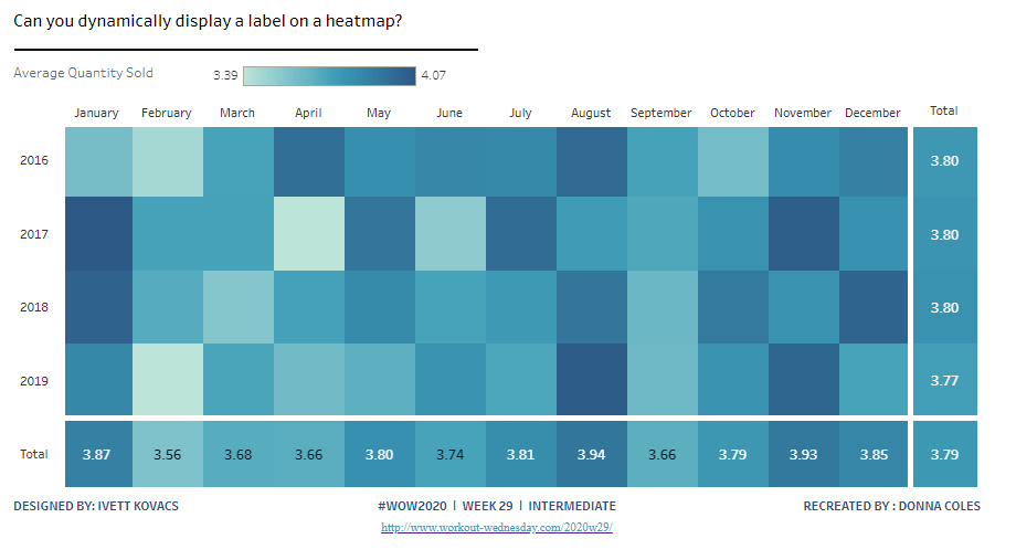
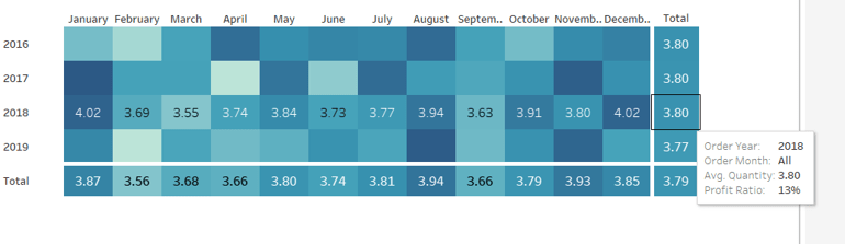
Ivett Kovacs returned with the #WOW challenge for this week, providing 2 versions. She provided some hints in the requirements which helped. With a bit of head scratching I managed to deliver an advanced version too. It didn’t exactly match what Ivett had delivered, but I was quite happy with my version. Until my follow #WOW participant Rosario Guana pointed out that the display ‘on click’ of a row or column total didn’t work properly 😦
I’ve spent A LOT of time trying to figure out what’s required but can’t resolve it. I’ve checked out Ivett’s solution and noticed a slight flaw in her logic too, so I feel uncomfortable changing my flaw for another. I’ve also looked at other solutions, and all are showing slightly different behaviour when you click on a column or row cell total. As a result, I’ve decided to blog based on the Intermediate version only. Others have posted blogs about their Advanced versions, so I’m going to save some time today, and reference them instead.
Building the basic heat map
The core of this challenge is going to involve Sets, and we’re going to use Set Actions to identify which cell is being interacted with.
For the intermediate version, we’re interacting based on hover actions.
The heatmap displays a grid of months by years, and we need to build sets based off of these. So we’ll start by creating dedicated calculated fields storing these values
Month Order Date
DATENAME(‘month’,[Order Date])
Year Order Date
YEAR([Order Date])
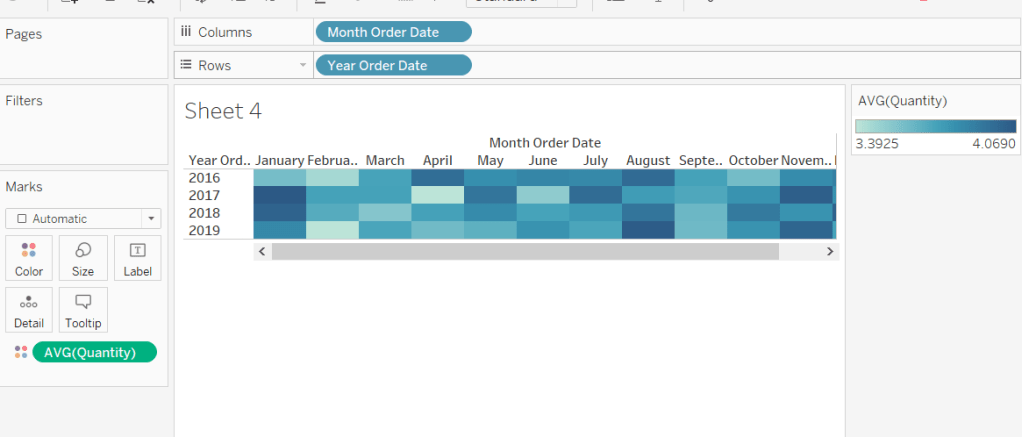
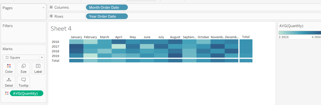
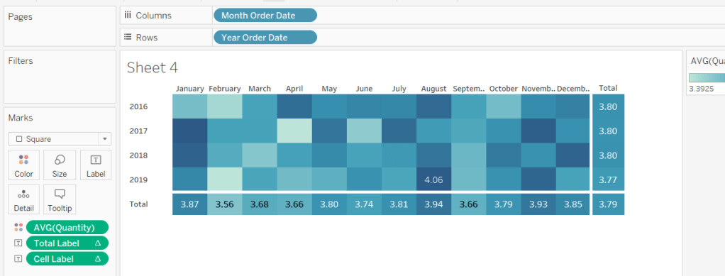
Add Month Order Date to Columns and Year Order Date to Rows, then drag Quantity onto Colour and change to AVG. You should have your basic heatmap.
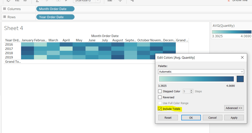
From the Analysis -> Totals menu, select to shoe row & column grand totals. They will initially display as white cells, so you need to Edit Colours on the colour legend and select Include Totals/
Let’s sort some formatting out at this point.
Set the mark type to Square
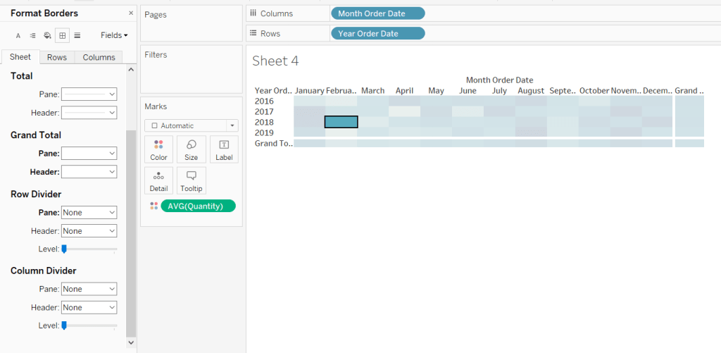
Format the borders by setting the row & column dividers to none, but setting the Grand Total pane & header to be thick, white lines
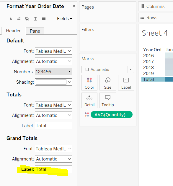
And change the word Grand Total, by right clicking -> format on each cell and changing the Grand Total label.
Adjust the size of the Month & Year labels and remove header labels from displaying and you have
Labelling the total cells
We need to permanently display the label on the total row/column, and only show the label on the cells ‘on hover’.
We need a way to identify when we’re on a total cell. Ivett gave a hint “What is the Size() of the totals and the cells?“. This is a trick I’ve read about and discussed here. Basically the size() of the grand total row or column will be 1, so this is what we’re going to base some logic on.
Size of Months
SIZE()
Size of Years
SIZE()
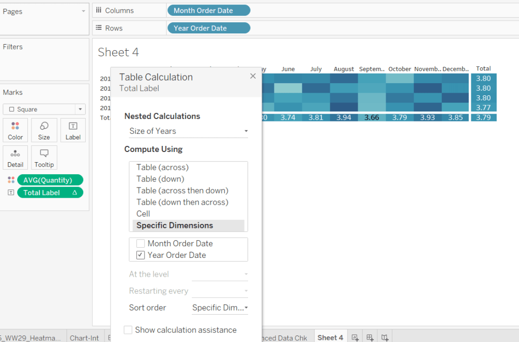
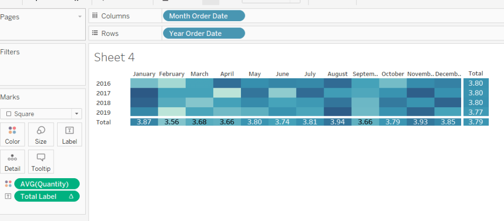
Total Label
IF [Size of Years]= 1 OR [Size of Months] = 1 THEN AVG([Quantity]) END
If we’re on a row or column grand total, then show the AVG(Quantity). Add this onto the Label shelf, and edit the table calculation so the Size of Years nested calc is computing by Year Order Date, and the Size of Months nested calc is computing by Month Order Date.
Labelling the central cells
We need to create some sets, as these are going to determine whether we are hovering on a cell or not. The dashboard action will add values to a set on hover.
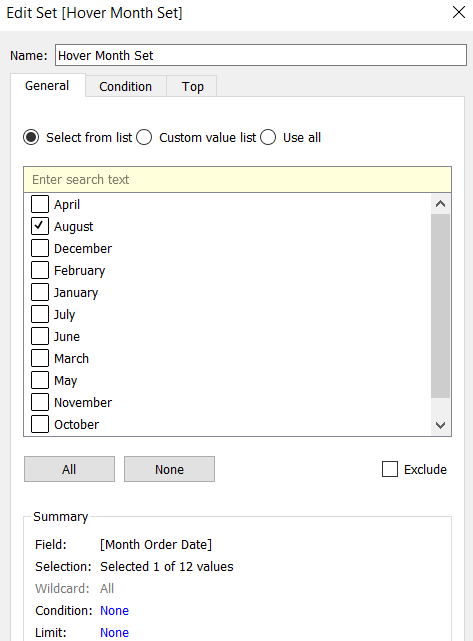
Right click on Month Order Date and Create Set, selecting an arbitrary month.
Hover Month Set
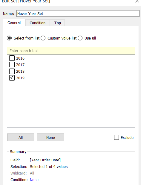
Do the same with Year Order Date
Hover Year Set
We then need a field to label the cell
Cell Label
IF ATTR([Hover Month Set]) AND ATTR([Hover Year Set]) AND [Size of Months]>1 AND [Size of Years]>1 THEN AVG([Quantity]) END
If something has been selected in the Hover Month Set and something has been selected in the Hover Year Set, and we’re not on a grand total row/column, then show the AVG(Quantity).
Add this to the Label shelf, and edit the table calculation settings as above.
Tooltip
The tooltip displays the Profit Ratio
SUM([Profit])/SUM([Sales])
so you’ll need to create this field, add to the tooltip and adjust the display accordingly.
Add the interactivity
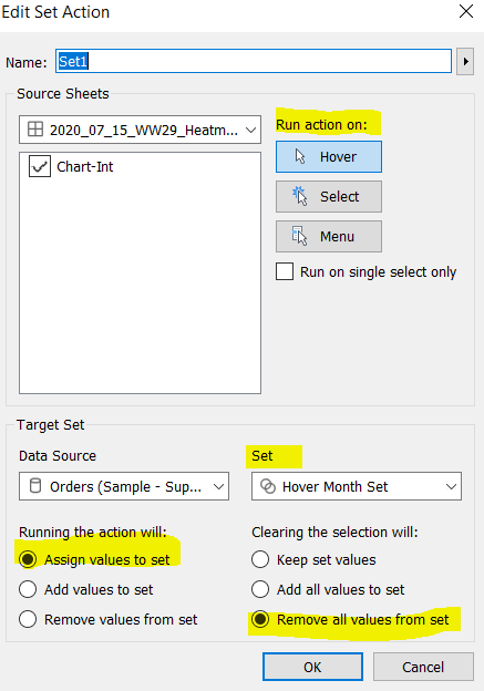
Add the above sheet onto a dashboard, then create a dashboard action to Change Set Values, which is set to
run on Hover
Target the Hover Month Set
Assign values to the set when run and remove values from the set when cleared
Repeat to create a set action to target the Hover Year Set.
Test it out – hover your mouse over the cells. If you hover on a total, you should get the values displayed for all the values in the row or column
Advanced Version
As I stated in the intro, I didn’t end up with something I was entirely happy with. While writing this up, I’ve tried to rebuild using ideas from other published solutions, but I still have got anything ‘perfect’.
Ivett’s solution is obviously the closest to what we’re aiming for, since that is the challenge. The minor flaw I found in that though was that in some of the labelling logic there’s a step which compares the ‘average of the selected cell’ with the ‘average of the current cell’, and if they match, display the AVG(Quantity), otherwise show the difference. This logic is basically trying to work out ‘if current cell = selected cell’, but it doesn’t fully work, as there are other cells where the values match – it’s subtle as the displayed values are faded out with the cell highlighting, as I’ve shown in the example below.
Kyle Yetter has blogged his solution here, but if you click on a row or a column total in his solution, the values are all the same, and not showing a difference.
Rosario Guana has blogged her solution here. Rosario has adapted her solution slightly and displays both the average values and the difference ‘on select’, so the logic I was struggling with, isn’t being used in the same way here.
No doubt with a bit more time, I might finally crack this one, but for now, I need to ‘put it to bed’ 🙂
This week’s #WOW challenge was set by Ann primarily to demonstrate the recent 2020.2 release of relationships in Tableau. This is a change to how the data modelling works when combining data together, in this case actual sales data and sales goal (target) data. Ann provided a ‘tweaked’ version of superstore sales data for the actual sales, alongside a custom ‘goals’ data set which provided a sales goal value for each month per Segment and Category (ie the goals data was not as granular as the actual sales data).
Combining the Data
Obviously, to make use of the new relationships feature, you’ll need at least v2020.2.1 installed.
When you add the 2 data sources to the Data Source pane and add the Orders sheet from the Superstore data and then add the Sheet 1 from the Sales Goals data, you’re prompted to add a relationship if matches can’t automatically be found (ie the field names aren’t identical).
I added relationships for the Segment, Category and Month of Order Date fields, which then provides a ‘noodle’ link between the two sets of data
Note – to add multiple relationships, you have to close the field listing to then see the Add more fields option.
With relationships, Tableau is now smarter at how it manages the queries between the data. I’m not going to go into it at length (as there’s plenty of good Tableau documentation on the subject), but I’ll quickly show the difference between this and a traditional ‘join’.
In the Relationships model, if I show Sales and Goal by Month & Segment, the Goal is based on the sum of the rows associated to that Month and Segment that you can find if you looked at the source spreadsheet directly
But if I was using a traditional join with these data sets :
and then presented the same info as above
The Goal data is way off, as it’s being influenced by all the additional rows of data that have been constructed by the join clause.
If we expand to the Category level in each example above (the level at which the Goal data is stored), the Relationship version still shows the correct value
while the Join version is still incorrect, and only changing to an Average aggregation do we get the figure needed
Joining the data requires more work (calculations / knowledge) to ensure the Goal data is reporting correctly at the various levels, whereas the Relationships model ‘just works’.
Building the Table
When I started building the solution, I actually started with the YoY trend chart, but found I had to revisit it (swap a couple of pills about) as I progressed through, so I’m going to start with the table of data itself.
This turned out to be really quite tricksy… it’s just a table right… looks harmful enough…. but Ann had lobbed a few ‘gotcha’ grenades into the mix, that took a bit of head-scratching!
First up, Ann likes to use capitalisation, so I simply renamed the following fields
Category (from Sheet 1 – the Goals data) -> CATEGORY
Segment (from Sheet 1 – the Goals data) -> SEGMENT
Month of Order Date (from Sheet 1 – the Goals data) -> MONTH
Sub-Category (from Orders – the Superstore Sales data) -> SUB-CATEGORY
And I then created a hierarchy called SEGMENT which stored SEGMENT – > CATEGORY -> SUB-CATEGORY.
We also needed to ‘fake’ today so we can show sales to date. The Orders Superstore data set contains data from the start of 2016 to the end of 2019. We needed to pretend ‘today’ was 1st July 2019 and not show any sales beyond the end of the month. So I created the field
Today
#2019-07-01#
and then
ACTUAL SALES
IF DATETRUNC(‘month’,[Order Date])<= [Today] THEN [Sales] END
If we build out the basics of the table
SEGMENT hierarchy on Rows
MONTH (discrete, exact date, formatted to mmmm yyyy) on Rows
Measure Names on Columns and on Filter, filtered to ACTUAL SALES and Goal
Measure Values on Text
MONTH on Filter, set to exclude 2016
we get
and as we expand the hierarchy to the next level, the ACTUAL SALES and Goal adjusts as expected
but when we reach the 3rd level we see a couple of issues
The Goal is showing the values that were displayed at the CATEGORY level, since it isn’t set at any further level. The requirement we have is to show the value ‘No Goal’ instead once we reach this point.
We also have a set of values with a NULL SUB-CATEGORY. This is because there are dates with goal values in the Goals data set, but we have no Sales data for those dates, so a match at the SUB-CATEGORY level can’t be found. We need to remove these records when at this level, and actually only show records where we have ACTUAL SALES, so records from July 2019 onwards should also be excluded.
At this point, I did end up having a sneak look at Ann’s solution. I had an idea of what I wanted to do, BUT I was worried that I may be missing something related to the new data model… that perhaps there was a feature of relationships that I needed to be exploiting as part of this, rather than go down the table calculation route I was heading towards. After all, part of doing these challenges for me is to make use of new features & functions if I can, so I have a reference workbook for future use. I had a read up on the blog posts related to relationships, but couldn’t spot anything obvious, hence a quick check at Ann’s solution…. nope nothing special required in respect of the data model….so instead, we need some additional calculations to help resolve all this.
What we need is some way to identify when we’re at the lowest SUB-CATEGORY level. We’ll start by counting the number of distinct sub-categories we have
# Sub Cats
ZN(COUNTD([SUB-CATEGORY]))
Wrapped in a ZN will return the value 0 when none exist.
Dropping this into the table of data, we can see the 0s for all the future Goal records, and 1 for the rest of the rows, since we’ve expanded to the SUB-CATEGORY level.
If you collapse up to the CATEGORY level, the #Sub Cats count changes, as each row typically contains more than 1 SUB-CATEGORY.
The term ‘typically’ in the above statement though is the reason we can’t assume we’re at the lowest level if the count is 1 though. It is possible for the sales against a particular CATEGORY in a MONTH to only span a single SUB-CATEGORY (Check out Home Office -> Furniture in Jan 2018). So we also need
Max Sub-Cats in Window
WINDOW_MAX([# Sub-Cats])
Which will count the maximum number of SUB-CATEGORY records for each SEGMENT and CATEGORY. In the case of Furniture Sales in the Home Office in Jan 2018, you can see below the count of sub-categories is 1 but the maximum count in the window is 4.
This shows we’re not at the SUB-CATGEORY level, as when we are, the #Sub Cats = Max Sub Cats in Window (ie 1=1)
So with that knowledge we can now derive an alternative field for the goal
SALES GOAL
IF ([# Sub-Cats] = 1 AND [# Sub-Cats]=[Max Sub-Cats in Window]) THEN 0 ELSE SUM([Goal]) END
Remove the original Goal field from the table and add this instead, setting the table calculation to compute by MONTH and you’ll see the SALES GOAL value change from a value to 0 as you expand down to the SUB-CATEGORY level.
So how do we show ‘NO GOAL’ instead of 0? Well this is a bit of a sneaky formatting trick, and one I couldn’t figure out (this step was actually the last thing I changed before publishing).
In my original SALES GOAL calculation I had set the value to be NULL rather than 0 expecting there to be an option to show the NULL values as something else (ie NO GOAL). But the feature I was looking for wasn’t available (maybe I was mistaken about when it appears.. maybe it’s disappeared in 2020.2… I still need to investigate). Anyhow, my alternative was to create a string field to store the value in, but this would make formatting the number quite cumbersome, and I was sure that wasn’t the case.
So I had to check Ann’s solution. Instead of NULL, she had set the value to be 0, and consequently used the following custom number formatting :
“$”#,##0;-“$”#,##0;”NO GOAL”
where the last bit is how to format 0. Very very sneaky huh!
So we’ve worked out how to identify when we’re at the SUB-CATEGORY level, and managed to display ‘NO GOAL’ when at that level, now we need to filter out some of the rows (but only when at this level).
Records to Show
IF [Max Sub-Cats in Window] = 0 THEN FALSE ELSEIF ([# Sub-Cats] = 1 AND [# Sub-Cats]=[Max Sub-Cats in Window]) THEN //at lowest level IF ATTR([MONTH]) < [Today] THEN TRUE ELSE FALSE END ELSEIF [# Sub-Cats] = 0 AND [Max Sub-Cats in Window] = 1 THEN FALSE //still at lowest level but no sales so exclude ELSE TRUE END
This took a bit of trial & error to work out, and there may well be something much more simplified.
Adding this to the table, and again setting to compute by MONTH you can see which rows are reporting True and False. When collapsed to the SEGMENT or CATEGORY level, all rows are True, but the values start to vary when at the SUB-CATEGORY level.
Now, we need to work on the fields to help show us the actual & % difference.
RESULT
IF ([# Sub-Cats] = 1 AND [# Sub-Cats]=[Max Sub-Cats in Window]) THEN NULL ELSE SUM([ACTUAL SALES])-([SALES GOAL]) END
The difference should only show if we’re not at the lowest level. This needs to be custom formatted as
will give me the % difference (format to percentage with 0 dp).
And the final piece of data we need (I think) is to compute a RAG status for each row. This is dependent on some parameters
GREEN (WITHIN X%)
Type Float, set to 0.1 but displayed as a percentage
and similarly
RED (ABOVE Y%)
With these we can work out
RAG
IF ABS([ACTUAL vs GOAL]) > [RED (ABOVE Y%)] THEN ‘WAY OFF TRACK’ ELSEIF ABS([ACTUAL vs GOAL]) < [GREEN (WITHIN X%)] THEN ‘ON TRACK’ ELSEIF ATTR([MONTH])>=[Today] THEN ‘NO COMPARISON’ ELSEIF [SALES GOAL]=0 THEN ‘NO COMPARISON’ ELSE ‘OFF TRACK’ END
If you add all these fields to your table then you can check how they all compare/change as you expand/collapse the hierarchy (make sure you set the compute by MONTH on all fields).
So now we’ve got all the building blocks you can create the actual table.
I’d recommend duplicating the above (and keeping as a ‘check data’ sheet). Then remove the fields you don’t need, and add the Records To Keep = True to the Filter shelf. Format the table appropriately, and add the title so you’re left with
Building the Line Chart
As mentioned above, I started with this chart, but ended up having to revisit it as I found I needed to use different pills that got created as I built the table. There is actually 1 additional field needed, which isn’t obvious until you start playing with the dashboard actions later:
GOAL
IF [SALES GOAL] > 0 THEN [SALES GOAL] END
This is needed so that when we filter by SUB-CATEGORY later and there is no goal, we only get a single line displaying the sales values, rather than also having a line plotted at 0.
MONTH on Filter, excluding Year 2016
MONTH (exact date, continuous) on Columns
Measure Values on Rows and Filtered to ACTUAL SALES and GOAL
Coloured accordingly by Measure Names
Then add TODAY to Detail and add a Reference Line to the MONTH axis, setting it to TODAY, adjusting the format of the line, and setting the fill above colour to grey.
Format the gridlines, tooltips & axis accordingly to match
Barcode / Strip Chart
For this we’re creating a bar chart using MIN(1), and fixing the axis to range from 0-1 so it fills up the entire space as follows
MONTH on Filter excluding Year 2016
MONTH as exact date, discrete (blue pill) on Columns
MIN(1) on Rows
RAG on Colour adjusted accordingly
ACTUAL vs GOAL on Tooltip
Then use the ‘type in’ functionality to create a pill labelled ‘vs Goal’ on the Rows
Creating the Dashboard
I used a vertical container to add the components onto the dashboard, as I used blank objects that are formatted with a black background, 0 padding and a height of 4 to create the horizontal line separators.
The interactivity between the table and the other charts is managed via Dashboard Filter actions.
To get these to work properly though, and in such a way that the selected SEGMENT and/or CATEGORY and/or SUB-CATEGORY can be referenced in the title of the line chart, 3 separate dashboard actions are required, with each one specifying the field to filter by, as follows :
Once these are set up, the associated pills will appear on the Filter shelf of the Line and Barcode charts, and are then available for selection when building the title of the line chart
Luke Stanke set the challenge this week, and posted a ‘sneak peak’ on Twitter before the challenge was formally released
Challenges from Luke can sometimes be on the harder end of the scale, so with the bit of extra time available and only the gif in the tweet as a clue , I had a play to see if I could get close at all. And surprisingly I could, so once it was formally issued, it was just a case of tidying up some of my calcs.
Calculations
First up we need to establish the basic calculations
Plotting these out onto a table with Segment we get
Note #Orders Per Customers needs to be set to be a discrete dimension.
So while this shows us a summary of the number of customers, we’ve only got 1 mark showing the summarised count. When plotting the chart we need something else in the view that will generate more marks. This is Customer ID.
At this point in order to help us build up our tabular view to ‘see’ what’s going on, I’ll filter the table to just show Segment = Consumer, and I’ll add Customer ID to Rows
As expected, our # Customers is now showing a count of 1 per row, but the data is now expanded as we have now got a row (ie a mark) per customer for each # Orders Per Customer ‘bucket’. But we still need a handle on the total customers in each ‘bucket’.
Customers Per Order Count
WINDOW_SUM([# Customers])
Adding this to the view and setting the table calc to compute based on Segment & Customer ID, we get the summarised value back again.
But we don’t want to actually show that number of marks; the number of circles to plot on the chart is dependent on a user parameter:
pMarkIndicator
Based on the requirements, if the number of customers is 15 and the user parameter is 5, then 3 circles should be drawn (15 / 5 =3 ), but if the number of customers was 14, only 2 circles should be drawn (14 / 5 = 2.8), ie the number of circles will always be set to the integer of the equal or lesser value (essentially the FLOOR() function). This can also be achieved by
Marks to Plot
INT([# Customers per Order Count]/[pMarkIndicator])
For some reason FLOOR can’t be used in the above as a table calculation is being used, but INT does the job just fine, and adding to the tabular view and adjust the table calculation accordingly we get
ie for the Consumer Segment, 6 customers have made 1 order in total, so based on batching the customers into groups of 5, this means 1 circle should be displayed. Whereas, 30 customers have made 3 orders in total, so 6 circles should be displayed.
But we can’t actually reduce the amount of rows (ie marks) displayed – we either have 1 row (by removing Customer ID) or a row per customer. But that’s fine, we don’t need to.
What we want is something in our data to group each row into the relevant batch size.
First up let’s generate an ID per row for each customer that restarts for each #Orders Per Customer.
Index
INDEX()
Add this as a discrete pill to Rows, and adjust the table calc
Now we have this, we calculate which ‘column’ each customer can sit in, a bit like what we would do if we were building a small multiple table, arranging objects in rows and columns (see here for an example of what I mean).
Cols
[Index]%([Marks to Plot])
This uses the modulo (%) notation which returns the remainder of the division sum. Lets put this on the view
For customers who have only ordered once, and where we’re only going to plot 1 mark, the Cols value is the same (0) for all rows.
Whereas for customers who have ordered twice, and where we want to plot 2 marks, the Cols value is either 0 or 1.
We’ve now got a value we can use to plot on an axis. We’re still going to plot a mark for each Customer ID, but some marks will be plotted in the same position, ie on top of each other, which therefore looks like just one mark.
Let’s show this more graphically, by duplicating the sheet, deleting some pills, moving some around, changing some to continuous, and setting the mark type to circle as below
Change the pMarksIndicator parameter and the number of circles will adjust as required.
So far, so good. We’ve got the right number of marks, it’s just not looking as nice and symmetrical as it should be.
We need to shift the marks to the left. But how far it shifts is dependent on whether we’ve plotted an odd or even number of marks.
If we have an odd number, the middle mark should be plotted at 0. If we have an even number the middle two marks should be plotted at -0.5 and +0.5 respectively. The calculation below will achieve this
Cols Shifted
IF [Marks to Plot]%2 = 0 //we’re even THEN [Cols] – ([Marks to Plot]/2) + 0.5 ELSE //we’re odd [Cols] – (([Marks to Plot]-1)/2) END
To demonstrate this, I’ve added Cols Shifted along side Cols on the viz (this time make sure all the table calculation settings (including the nested calcs) are applied to compute based on Customer ID only which is different from the calcs above)..
Now you can see how it all works, you can remove the Cols and the Segment from the Filter shelf.
And now its just a case of applying the various formatting to clean up the display, and adding to the dashboard.
Guest poster Ivett Kovacs was back to set the weekly #WOW2020 challenge this week, and delivered a very ‘relatable’ business challenge – Fiscal Year to Date reporting.
I’ve been quite used to doing this type of reporting within my job, so on the whole I found the core requirements pretty straightforward – there’s just a lot of calculated fields 🙂 The trickiest part I found was getting everything organised on the dashboard and making the budget parameters appear/disappear based on the filter selected – this took an extraordinarily looonnnng time even though I knew the technique – more on that later.
Setting up the Fiscal Year
The data source provided was one curated by Ivett. It contained financial ‘transactions’ against Account Codes from Oct 2018 to May 2020.
The date in the file was initially recognised by Tableau as a string, but simply changing it to a Date datatype in the Data Source pane easily resolved this.
The fiscal year starts on 1st October, so once on a sheet, set this by right-clicking on the Accounting Date field and choosing Default Properties -> Fiscal Year Start -> October
If you add Accounting Date to a sheet and expand from Year -> Month, you’ll see that the Year part is now labelled as FY 2019 and FY 2020, and Q1 starts in October
Just a couple of points to be aware of if you’re not familiar with working with Fiscal Years.
A relative date filter for ‘this year’ will recognise your fiscal date setting, so if you did this on this data set, you’d get data from Oct 2019 to May 2020.
Any date related functions such as YEAR([Date]) or DATETRUNC(‘year’, [Date]) does not recognise the fiscal year setting. So YEAR(#2019-11-01#) will return 2019 and YEAR(#2020-01-01) will return 2020 even though they are both in the same FY 2020 fiscal year. It does mean at times, depending on what you’re building, you may need to hard-code information that defines the start month of your fiscal year.
Building all the calculated fields
First up we need a couple of measures as stated in the requirements.
Sales
IF STARTSWITH([Account Number],’5′) THEN [Value] END
only counts for Account Number starting with a 5
OPP
IF STARTSWITH([Account Number],’5′) OR STARTSWITH([Account Number],’696′) THEN [Value] END
only counts for Account Numbers starting with a 5 or 696.
Then we need lots of fields to help us get all the various data needed. This is simply going to be a big list 🙂
finds the maximum date in the dataset and sets to the 1st of the month, in this instance it will be 01 May 2020. This is a more generic approach than harcoding.
FY Start Current Year
#2019-10-01#
I said there might need to be some hardcoding! Ideally, having set a fiscal year, you’d like a function along the lines of DATETRUNC(‘fiscal year’, [Date]) to give you this value. Apart from setting this value in a parameter, I’m not aware of any way you can determine this date without any sort of hardcoding 😦 This KB article tries to provide some suggestions, but you still need to hardcode a value to ‘shift’ to the appropriate month; in this case we’d have to hardcode 10 as October is the 10th month. Feel free to upvote this idea on the Tableau Forums which asks to address this 🙂
Current FYTD Sales
IF DATETRUNC(‘month’,[Accounting Date]) >= [FY Start Current Year] AND DATETRUNC(‘month’,[Accounting Date])<=[Current Month] THEN [Sales] END
only return sales values for dates from 01 Oct 2019 to 31 May 2020.
Current FTYD OPP
IF DATETRUNC(‘month’,[Accounting Date]) >= [FY Start Current Year] AND DATETRUNC(‘month’,[Accounting Date])<=[Current Month] THEN [OPP] END
as above but for the OPP measure.
Current Month Prev FY
DATE(DATEADD(‘year’,-1,[Current Month]))
go back 1 year to 1st May 2019.
Prev FYTD Sales
IF DATETRUNC(‘month’,[Accounting Date])<= [Current Month Prev FY] THEN [Sales] END
Only return sales values for dates up to 31 May 2019. Note the data only starts from 01 Oct 2018, which is the start of the previous FY, but if we couldn’t guarantee that, we’d have stored an ‘FY Start Prior Year’ and added an additional clause to the above calculation.
Prev FYTD OPP
IF DATETRUNC(‘month’,[Accounting Date])<=[Current Month Prev FY] THEN [OPP] END
To deal with the Budgets, we need to create a couple of parameters Budget Sales (M) and Budget OPP (M). Both are integer parameters defaulted to 2,300 and 3000 respectively.
But because these parameters aren’t actually in millions, we need further fields to translate them into the value we really need for comparisons.
We need the MIN() function as the same Budget Sales Ref Line value is stored on every row, so SUM() will multiply the value too much. AVG() or MAX() would have worked just as well.
Curr vs Budget Sales Diff %
[Curr v Budget Sales Diff] / MIN([Budget Sales Ref Line])
and again we need to duplicate these for the OPP measure
Curr vs Budget OPP Diff
SUM([Current FYTD OPP]) – MIN([Budget OPP Ref Line])
Curr vs Budget OPP Diff %
[Curr v Budget OPP Diff] / MIN([Budget OPP Ref Line])
Now we’ve got all the core variables we need, we need to determine which one to use as the comparison in the bar chart and the KPI indicator. This is based on a parameter for the user to decide if they’re comparing Actuals against Budget or against Previous Year Actuals.
Compare Filter
I chose to create an integer based parameter with the display altered to show the relevant text. We will be using this parameter in calculated fields and comparing integers rather than strings is much more efficient (and easier to read).
So with the parameter set up, we now need to create a few fields that we’ll use to show the values we want
Sales Diff
IF [Compare Filter] = 0 THEN [Curr v Budget Sales Diff] ELSE [Curr v Prev Sales Diff] END
This is custom formatted to display as $ in millions with an arrow to show positive or negative : ▲”$”#,##0,,M;▼”$”#,##0,,M
Sales Diff %
IF [Compare Filter] = 0 THEN [Curr v Budget Sales Diff %] ELSE [Curr v Prev Sales Diff %] END
This is formatted to 1 decimal place.
Opp Diff
IF [Compare Filter] = 0 THEN [Curr v Budget OPP Diff] ELSE [Curr v Prev OPP Diff] END
Same custom formatting as above.
Opp Diff %
IF [Compare Filter] = 0 THEN [Curr v Budget OPP Diff %] ELSE [Curr v Prev OPP Diff % ] END
Sales Ref Line
IF [Compare Filter] = 0 THEN MIN([Budget Sales Ref Line]) ELSE SUM([Prev FYTD Sales]) END
This is used for the line shown on the bar chart, and we’ll need the same for the Opp measure.
Opp Ref Line
IF [Compare Filter] = 0 THEN MIN([Budget OPP Ref Line]) ELSE SUM([Prev FYTD OPP]) END
Finally we need a couple of fields to use to work what colour the bars need to be.
Colour : Sales Diff
IF [Sales Diff %] <-0.05 THEN ‘Difference < -5%’ ELSEIF [Sales Diff %] > 0.05 THEN ‘Difference > 5%’ ELSE ‘-5% <= Difference <= 5%’ END
Colour : OPP Diff
IF [OPP Diff %] <-0.05 THEN ‘Difference < -5%’ ELSEIF [OPP Diff %] > 0.05 THEN ‘Difference > 5%’ ELSE ‘-5% <= Difference <= 5%’ END
Note – my published solution has something slightly longer winded as when I originally built the viz, I created the colour fields before I created the generic Diff/Diff% fields referenced above.
Right! That’s a LOT of calculated fields (I did warn you!). In some cases it may have been possible to combine, but I like creating building blocks to keep things simpler to read.
Sales YoY Trend Line
The basis of this type of chart is pretty much Desktop 101.
Month(Accounting Date) on Columns (blue pill)
Sales on Rows
Year(Accounting Date) on Colour with colours adjusted accordingly.
Add the average line and Label the most recent point
Format the gridlines/rows etc and axis
The most recent mark is a larger circle. We need another calculated field for this
Current Month Sales
IF DATETRUNC(‘month’,[Accounting Date]) = [Current Month] THEN [Sales] END
This just stores the sales value for the latest month.
Add this field to the Columns and make dual axis and synchronise axis. Adjust the marks back to be a line and a circle and adjust the Sizes to suit.
Duplicate all the above on another sheet for the OPP values instead.
Sales Bar Chart
Simple bar chart
Current FYTD Sales on Columns
Colour : Sales Diff on Colour
Sales Ref Line on Detail
Add Sales Ref Line as a reference line and label & format to suit.
Label bar and align middle right; format to suit.
The colour legend will only display a single option at a time. You’ll need to set the Compare Filter to compare against budget and show, then adjust, the value of the Budget Sales (M) parameter to values that go beyond the thresholds, to set the other colour options.
Repeat all this again on another sheet for the bar displaying the OPP measure.
Sales KPI
Simply add Sales Diff & Sales Diff % to the Text.Format row/column lines to suit.
Again, repeat for the equivalent OPP measures.
Year Legend
The standard legends aren’t used as these are only square icons, but the challenge shows circles. So a custom legend sheet is created as below
The hidden axis has been fixed from 0.45-1 to push the display to the left more.
% Diff Indicator Legend
Again the standard legend can’t be used this time, as only 1 option ever shows. So this is a custom ‘fake’ legend.
I simply used the Account Number field for this purpose. I filtered a sheet to just 3 different Account Numbers. I then built a similar viz to the above, but using Account Number throughout.
The sneaky trick I used here was to simply ‘alias’ the actual Account Numbers displayed to the text I wanted.
Building the dashboard
Getting all the objects in the right places can be a bit of trial and error. All the objects on my dashboard, apart from the Budget parameters, are tiled using a mix of horizontal and vertical containers, nested within.
Hide/Show the Budget Parameters
This probably took me the most time. It’s using a technique sometimes referred to as Parameter Popping. It uses containers and works similarly to sheet swapping.
I had to build a ‘blank’ sheet for this – a sheet that will show (a blank value) and hide based on the Compare Filter parameter.
I needed another field
Is Prev Value to Compare
[Compare Filter]=1
This returns true if the parameter is set to compare against the Previous Year rather than the Budget.
This is added as a Filter to the blank sheet and set to True, which means the sheet will ‘show’ when comparing to Previous Year, and hide when comparing to Budget.
A floating horizontal container is then added to the sheet, and all the objects – the Budget parameters, some Text boxes to label the parameters and the ‘blank’ sheet are ‘carefully’ added. The blank sheet should be the first object on the left. I say ‘carefully’ as it took a lot of trial and error to make it work. If it is done right, then changing the Compare Filter parameter should make the budget parameters move left & right as the blank sheet shows and then hides.
The floating horizontal container is made wider than the dashboard itself, so the showing of the ‘blank’ sheet, pushes the other objects so far to the right that they’re not on the dashboard at all.
The screen shots below show what it looks like in Desktop
As I said, Parameter Popping can be a bit tricky – I only used it twice, so haven’t yet found a sure fire way to get it right first time. If you google ‘Tableau Parameter Popping’ you’ll find a few links that might help, and/or check out Week 4 of #WOW2020 which also uses it (the other time I’ve used it).
And that’s about it. My published viz is here. Enjoy!
Lorna set a fun ‘create your own pizza’ challenge this week to demonstrate the ability to both add and remove items in a set via the use of Set Actions, a feature introduced in v2020.2 (so you’re going to need this to complete the task).
There’s essentially 5 components to this dashboard, which I’ll guide you through
The central bar chart
The graphical product type selector on the left
The list of selected products to the right
The actual vs budget bar at the top
An indicator of how much you’re over/under budget
Central Bar Chart
The essence of this is a simple Type, Product by Price bar chart, coloured by Type. Manually move the Type field so the ‘Size’ option is at the top.
To indicate if the product is vegetarian or not, we create
Veg Indicator
IF [Vegetarian] = ‘Yes’ THEN ‘●’ ELSE ” END
which we can add to the Row shelf, and format to be coloured green (I use this site to get the shapes).
The tick is used to indicate if the product has been added to the pizza or not. Selected items will be identified by the use of a set, so we need to create one. Right-click Product and Create->Set. Tick a few options.
And similar to the Veg Indicator we can build
Selected Product Indicator
IF [Selected Products] THEN ‘✔’ ELSE ” END
Add this to the Row shelf between Type and Product.
The order of the Products listed will change. I want it to be orderedalphabetically by Product within each Type. The quickest way to resolve this, was to duplicate the Product field, add it to the Rows between the Type and Selected Product Indicator pills, and then hide it.
The final requirement for this chart, is to highlight the selected products in a different shade of the ‘base’ colour.
Add Selected Products to the Detail shelf, then change the … detail icon to the left of the pill to the colour icon. This will mean there are 2 pills on the Colour shelf, and the colour legend will change. Adjust to suit
The chart just then needs formatting to add the Price to the Label of the bar, remove the row/column lines, hide the Type column, hide the field labels, hide the axis, and adjust the width of the columns.
Product Type Selector
Lorna provided the images needed for this, which need to be saved to a new folder in the Shapes directory of your My Tableau Repository. I called my new folder simply Custom.
Then on a new sheet, add Type to Rows, set mark type to Shape and add Type to shape too.
Hide the Type heading and remove the row lines.
Selected Products List
Add Type & Product to Rows and enter MIN(1) onto the Columns. Add Selected Products to the Filter shelf to restrict the list just to those in the set.
Add Type to Colour and Product to Label, changing the font to white and centring. Fix the axis from 0-1 and hide it. Hide the Type & Product columns.
Manually reorder the Type field to be listed Size -> Crust -> Sauce -> Toppings
Actual vs Budget Bar
The budget field can be changed by the user, so we need a parameter, Budget, for this, which is an integer parameter where the display is formatted to £ with 0dp, and defaulted to 15.
Create the bar by adding Price to Columns, Selected Products to Filters and Type to Colour. Reorder the items in the colour legend to get the colours displaying in the correct order with ‘Size’ on the left and ‘Toppings’ on the right.
Add the Budget parameter to the Detail shelf, then add a Reference Line which refers to the Budget. Adjust the label displayed to be custom as shown below, and format the thickness and colour of the line to suit
Format the reference line so the text is displayed at the top right, and edit the font & size of the label displayed.
Then make the row height of the chart taller, but adjust the size of the bar to be narrower. The reference line spans the whole height of the row, so reducing the height of the bar itself provides space for the label to display without overlapping the bar.
Hide the axis and remove gridlines etc.
Finally we need to display the total price of the products selected. We can’t just add Price to Label as there are multiple segments on the bar, and this will display a Price per Type.
Instead we need a new field
Total Price Selected Products
{FIXED [Selected Products]:SUM([Price])}
Since this chart is filtered by Selected Products = True, this returns the total price of all the items in the set (selected). Add this to the Columns shelf and make dual axis & synchronise axis.
Readjust the mark types, so the Price marks card is back to a bar, and the Total Price Selected Products is Text. Remove the Measure Names pill from the Colour shelf of both cards (the dual axis will have automatically added it), and also remove the Type pill from the Colour shelf of the Total Price Selected Products card. Instead, add Total Price Selected Products to the Text shelf of this card.
The text will overlap the bar whether you align left , middle or right. The trick is to add some spaces in front of the text and then align right.
Hide the axis.
Over / Under Budget Indicator
This is just a text display, but a few calculated fields are needed so the text can be coloured differently depending on whether it’s over or under.
First we need to know the difference from budget
Diff from Budget
[Budget]-[Total Price Selected Products]
Text Budget Diff Over
IF [Diff From Budget] < 0 THEN ABS([Diff From Budget]) END
This will just display the difference if the value is negative, but the ABS function will return the number as a +ve. This field should be formatted to £ with 2 dp.
Text Budget Diff Under
IF [Diff From Budget] >= 0 THEN [Diff From Budget] END
This will just display the difference if the value is positive. Format to £, 2 dp.
Only one of these fields will ever hold a value at any time.
Similarly we need fields to show the text to display.
Over Budget Text
IF [Diff From Budget] < 0 THEN ‘Over Budget’ END
Under Budget Text
IF [Diff From Budget] >= 0 THEN ‘Under Budget’ END
On a new sheet, add Selected Products to the Filter shelf, then add all four of the above fields to the Text shelf.
Adjust the order and colour of the fields in the Label editor, setting the fields related to being ‘over budget’ to red and the ‘under budget’ fields to green.
Now we’ve got all the building blocks, we can put it all on a dashboard.
Building the dashboard interactivity
Add all the sheets in their various locations. Most were tiled, except for the Budget parameter and the Over/Under Budget Indicator sheet, which I floated.
Filter the bar chart
Add a dashboard Filter Action to filter from the Type Selector sheet to the Product Bar Chart on select, filtering on the Type field only.
Add / Remove from Set
Add a dashboard Set Action to the Chart sheet that runs from the Menu, and adds the selected item to the Selected Products set.
Create another Set Action on the same chart, which removes values instead.
And that’s the main crux of the challenge. The only addition is ‘nice’ feature to avoid the item selected from being shown as selected (ie fading out all the other items in the chart).
I reverted to the trusty true = false dashboard action which I applied to the Selector chart and the Selected Items chart.
This involves creating 2 new fields True = True and False = False and adding these to the Detail shelf of the relevant chart.
A dashboard Filter action is then added which targets itself using the fields True = False
However, when I tried to add this same feature to the main bar chart itself, the bar chart stopped working as expected. I think there was conflict between there being 2 filter actions on the same chart. I have to admit, this is where I did check Lorna’s solution, as this was a small feature that really bothered me, and I didn’t want to publish without it.
It turns out she simply used a highlight action to resolve this
I vaguely recall using this sometime ago, but the ‘true=false’ concept has become so ingrained as my ‘go to’ method, that I struggled to think of this.
And that should be it. You now have the tools to customise your own pizza 🙂