What happens if? Can you update sales forecast and targets using only parameters?

So after Ann’s gentle workout for week 6, newly crowed Tableau Zen Master Lorna, hit us with this challenge, and I confess, I struggled. The thought of then having to write this blog about it even brought a little tear to my eye 😦

But here I am, and I will do my best, but I can’t promise I understood everything that went on in this. I truly am amazed at times how some people manage to be so creative and bend Tableau to their will. It really is like #TableauBlackMagic at times!

So I read the challenge through multiple times, played around with Lorna’s published viz, stared at the screen blankly for some time…. I found the University Planning Dashboard viz by Ryan Lowers that Lorna had referenced in the challenge as her inspiration (she’d linked to it from her published viz). I played around with that a bit, although that took a while for me to get my head round too.

I also did a google search and came across Jonathan Drummey‘s blog post : Parameter Actions: Using a parameter as a data source. This provided a workbook and some step by step instructions, so I used this as my starting point. I downloaded the workbook, copied across the fields he suggested and tried to apply his instructions to Lorna’s challenge. But after a couple of hours, it felt as if I was making little progress. I couldn’t figure out whether I needed 2 or 4 parameters to store the ‘list’ data source variables (one each to store the list of selected categories for forecast, the list of selected categories for target, the list of selected forecast values, and the list of selected target values, or one each to store the list of selected categories and forecast values combined, and selected categories and target values combined). Suffice to say I tried all combos, using a dashboard to show me what was being populated on click into all the various fields/parameters I’d built. But it just wasn’t giving me exactly what I needed.

I downloaded the University Planning Dashboard and tried to understand what that was doing. And finally I shrugged my shoulders, and admitted defeat and cracked open Lorna’s solution. When I finally get to this point in a challenge, I try just to ‘have a peak’, and not simply follow verbatim what’s in the solution. I gleaned that I did need only 2 parameters, and that what I had been doing with my attempts with Jonathan’s example was pretty close. It made me feel a bit better with myself.

How things then transpired after that I can’t really recall – it was still a lot of trial and error but I finally got something that gave me the Sales Forecast data and associated select & reset functionality (by this time I’d probably spent 4 hours or so on this over a couple of evenings). Once I’d cracked that, the target was relatively straight forward, so by the time I’d finished on the 2nd day, I had a dashboard that allowed the selections/resets and simply presented the data in a table on screen. I chose to keep that version as part of my published solution, just for future reference (see here). I then finished off the next day, building the main viz.

What follows now, is just an account of the fields etc I used to build my solution. So let’s get going….

Building the Sales Forecast Selector

I’m going to start by focusing on building the left hand side of the viz, setting and resetting the Sales Forecast values for each Category.

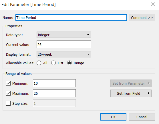
We need 2 main parameters to start with:

Forecast Param

An integer parameter defaulted to 70,000. This is the parameter that stores the value of the forecast to set.

Forecast List

A string parameter defaulted to empty. This is the parameter which will ‘build up’ on selection of a category, to store a delimited list of category + forecast values – ie the data source parameter.

Oh, and I also used a 3rd parameter, Delimiter, which is just a string parameter storing a :

The delimiter needs to be a distinct character that mustn’t exist in the fields being used. The Category field nor the Forecast Param field will contain a ‘:’, so that’s fine. But any other unused character would work just as well. Having this field as a parameter isn’t ultimately necessary, but it makes it easy to change the delimiter to use, if the chosen value doesn’t end up being suitable. It was also a field used in Jonathan Drummey’s solution I’d based my initial attempts on.

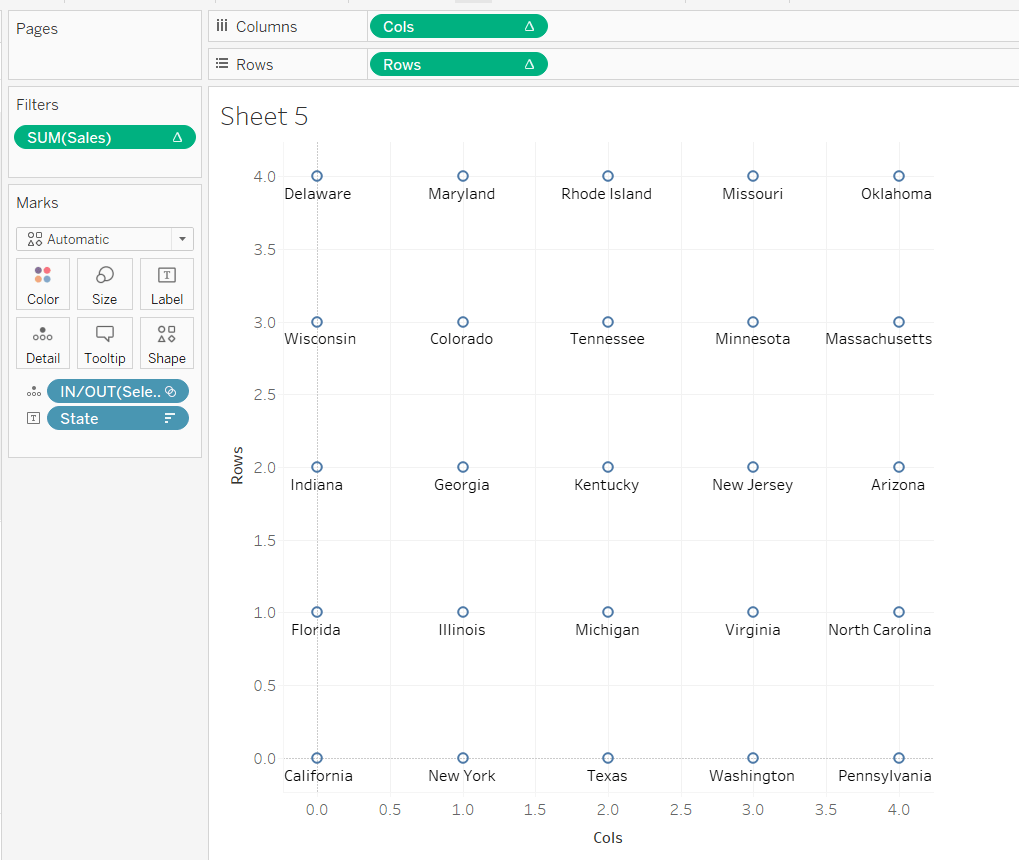
Now we need to build the viz to work as the category selector.

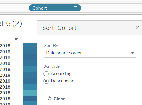
I simply put Category on the Rows shelf, sorting the pill by SUM(Sales) descending and set the Mark Type to circle. Oh – and I set a Data Source Filter to set the Order Date just to the year 2019.

I also needed the following

  • something to colour the circles based on whether the Category was selected or not
  • something to use to help ‘build up’ the List parameter ‘data source’
  • something to return the forecast value that had been selected against the specific Category

Category Exists in Forecast List

CONTAINS([Forecast List], [Category])

If the Category exists within the Forecast List string of text, this field will return true, and indicates the Category has been ‘selected’. This field is added to the Colour shelf, and the colour needs to be adjusted once parameter action has been applied to distinguish between true & false.

Add to Forecast List

if [Forecast Param]<>0 THEN
[Forecast List] +
[Category] + ‘_’ + STR([Forecast Param]) + [Delimiter]
ELSE ”
END

If the entered Forecast value isn’t 0, then append <Category>_<Forecast Value>: to the Forecast List parameter. Eg if the Sales Forecast value is $50,000 and Technology is selected, then Technology_50000: is added to the existing Forecast List parameter, which has started as blank.

If the Sales Forecast value is then changed to $10,000 say, and Office Supplies is selected, then the Forecast List parameter will become

Technology_50000:Office Supplies_10000:

This Append To Forecast List calculated field is used in conjunction with the Forecast List parameter within a Parameter Action on the dashboard to make all the ‘magic’ happen. The Append To Forecast List field must be in the view to be available to the parameter action, so it is added to the Detail shelf.

When a circle is selected the Append To Forecast List field is used to ‘set’ the Forecast List parameter, subsequently building up a string of Category_Value pairs.

Finally, on hover, the Category and the value of the selected sales forecast at the time must be visible on the Tooltip. To get the value at the point of selection, which isn’t necessarily the latest value visible in the Sales Forecast parameter displayed on screen, the following field is required:

Current FC Value

INT(if contains([Forecast List],[Category]) then
REGEXP_EXTRACT([Forecast List],[Category]+”_(-?\d+)”)
end)

This manages to pull out the number associated with the Category, so in the above example, would return 50000 for Technology and 10000 for Office Supplies.

This field has custom formatting applied : ▲”$”#,##0;▼”$”#,##0 and is added to the Tooltip shelf.

RegEx is a concept I have yet to really crack, so there is no way I’d have come up with the above on my own. I think it’s looking for the named Category followed by Underscore (_) followed by either 1 or no negative sign (-) followed by some numbers, and returns just the numeric part.

Finally, the circles shouldn’t be ‘highlighted’ when selected on the dashboard. To stop this from happening a calculated field of True containing the value True, and a field False containing the value False are required. These are both added to the Detail shelf, and a Filter Action is then required on the dashboard setting True = False. This is a technique that is now becoming a familiar one to use, having been used in earlier #WOW2020 challenges.

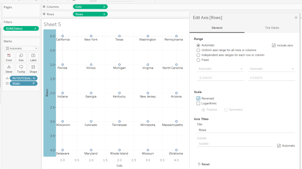
So my ‘selection’ sheet looks like

and when added to the dashboard, the parameter action looks like :

with the filter action looking like :

At this point, I’d suggest using a ‘test’ dashboard which contains the selection sheet, displays the Forecast List and Forecast Param, and has the dashboard actions described above, applied to get an idea of what’s going on when a circle is selected, and the values of the Forecast Param changed.

The final part to this set up, is the ‘reset’ button, which when clicked on, empties the Forecast List parameter.

Create a new sheet, change the Mark Type to Text, and on the Text shelf add the string ‘↺’. I simply typed this ‘into’ a pill, but you could create a calculated field to store the ‘image’, which isn’t actually an image, but a special string character, that I got off my favourite ‘go to’ unicode characters website.

You then need a calculated field

Forecast List Reset

that just contains an empty string. This is added to the Detail shelf.

Put this sheet on the ‘test’ dashboard, and create another parameter action

This takes the value out of the Forecast List Reset field and sets the Forecast List parameter, subsequently resetting the list to an empty string on click.

Verify this is all working as expected.

Building the Sales Target Selector

Subject to Sales Forecast selector working as expected, then apply exactly the same principles to create the Target selection sheet and associated parameters.

The only slight difference with the fields used in the Target selection is:

Add to Target List

if [Target Param]>0 THEN
[Target List] +
[Category] + ‘_’ + STR([Target Param]) + [Delimiter]
ELSE ”
END

This just applies the addition to the list if the entered target is a +ve number (ie > 0), rather than not 0 as in the forecast selection.

The Target also needs to be displayed on the Tooltip, and this time there is a default target value that should be displayed, even when no selection has been made. For this I created

Target

IF ZN(MAX([Current Target Value])) = 0 THEN
MIN(IF [Category]= ‘Furniture’ THEN 270000
ELSEIF [Category]= ‘Office Supplies’ THEN 260000
ELSEIF [Category]= ‘Technology’ THEN 250000
END)
ELSE MAX([Current Target Value]) END

which was formatted to a currency of 0 decimal places, prefixed by $. This was added to the Tooltip shelf.

At this point, you should now have both the ‘selection sheets’ working on the dashboard, so we can now focus on building the main viz.

Building the Bar Chart

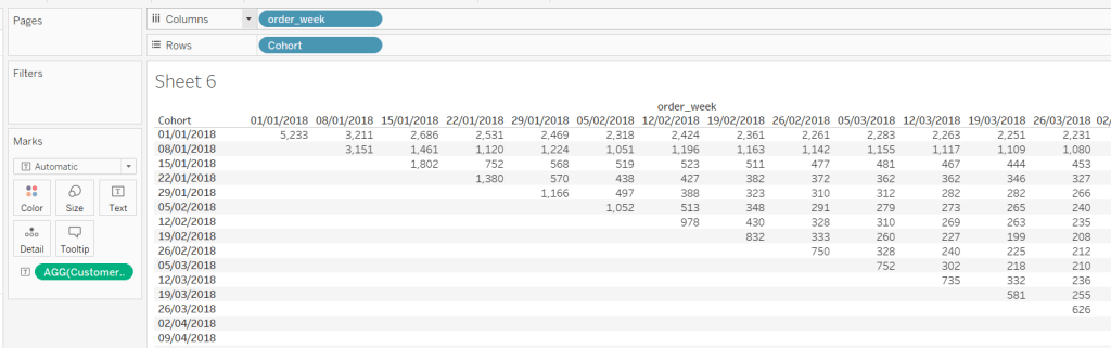
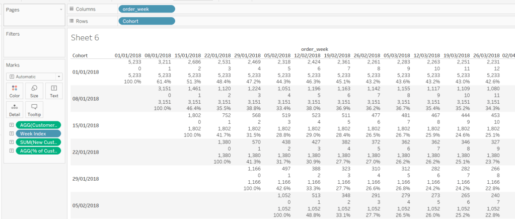
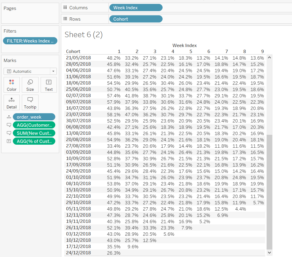
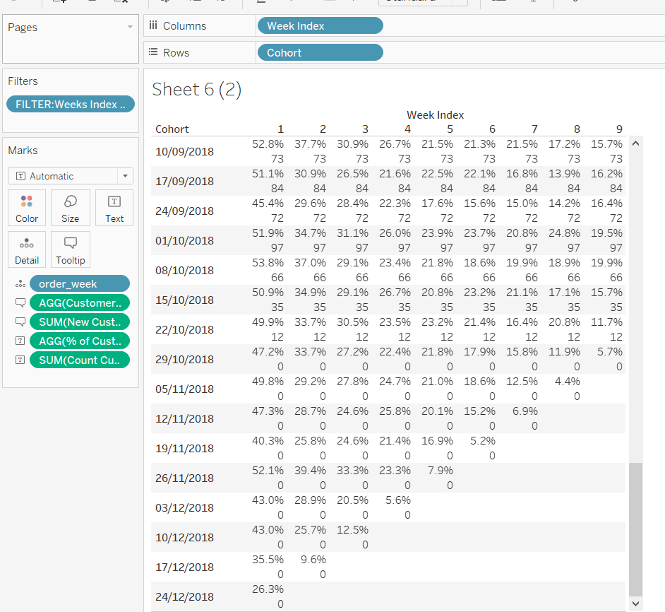
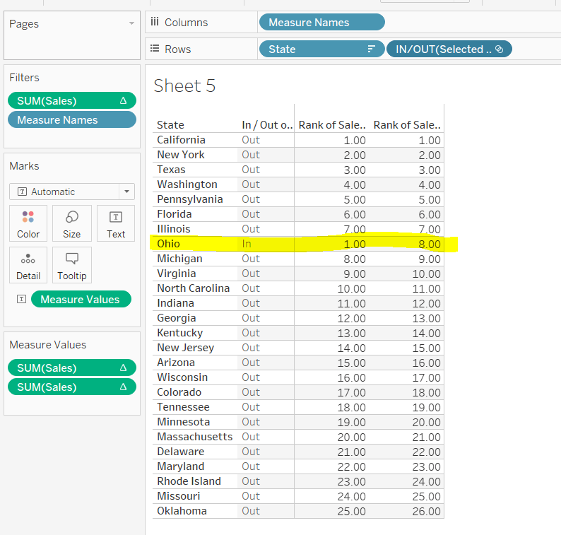
Rather than building the bar chart, I first decided to build a tabular view that simply presented on screen all the bits of data I needed for the bar chart, this being

  • Sales value per Category (simply SUM(Sales))
  • Sales Forecast value per Category (ie Sales + selected Forecast value)
  • Selected Sales Target value per Category (this is the Target field described above)
  • % Difference between Sales & Target
  • % Difference between Sales Forecast & Target

So I created the following additional calculated fields:

Forecast

SUM([Sales]) + MAX([Current FC Value])

formatted to currency prefixed with $ set to 0 dp.

Forecast vs Target Diff

([Forecast]-[Target])/[Target]

custom formatted to ▲0%; ▼0%

Sales vs Target Diff

(SUM([Sales])-[Target])/[Target]

also custom formatted to ▲0%; ▼0%

Adding the table to the ‘test’ dashboard allows you to sense check everything is behaving as expected

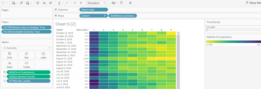
Now its just a case of shifting the various pills around to get the desired view. Ensure at least one Sales Forecast Category has been selected, to make it easier to ‘see’ what you’re building.

Lorna stated the target should be displayed as a Gantt mark type, with the sales and the forecast displayed as bars. This means a dual axis chart is required, with sales & forecast on one axis and target on the other.

To get Sales and Forecast onto the same axis, we need to add Category to the Rows (sorted by Sales desc) and Measure Values to the Columns, filtering to only the two measures we need.

Set the Mark Type to bar, and add Measure Names to both the Colour and the Size shelf.

Adjust colours and sizes to suit.

You might have something like


where the measures are ‘stacked’, so the bar is the length of the Sales then the length of the Forecast. We don’t want this, so need to set Stack Marks to Off (Analysis menu -> Stack Marks -> Off).

Add all the necessary fields to the Label shelf and format accordingly (you may need to widen the rows to make the labels show against each row).

Note – in my solution I created some fields to make the opening & closing bracket around the Forecast v Target Diff value only show when a Forecast had been selected, however in writing this blog, I realise it was simpler just to change the formatting of the Forecast v Target Diff to add the brackets around the number. The custom formatting was changed to : (▲0%); (▼0%)

Adjust the Tooltip to suit too.

Now add Target to Columns alongside Measure Values. Set to Dual Axis and Synchronise the axis. Reset the Measure Values mark type back to bar if needed, and set the Target mark type to Gantt.

Remove Measure Names from the Colour and Size shelf of the Target marks card. Untick Show Mark Labels too. Adjust the colour of the mark to suit, and you should pretty much be there now…

Tidy up the final bits of formatting, removing/hiding the various axis, labels, gridlines etc etc.

When this is all put together on the dashboard, you might need to fiddle about a bit with layout containers to get the bar chart lined up with the Selector views.

And with that I’m done! My published version is here, along with the ‘check’ dashboard I used to sense check what was going on, as I’m sure if I ever looked at my solution again, I’d struggle to understand immediately 🙂

Once again, I just want to acknowledge those that manage to create this magic with Tableau. I applaud you!

Happy vizzin’!

Donna

Can you build a MoM Progress Report?

Ann set the challenge this week, which for seasonsed #WoW participants like myself, was relatively straightforward. However it encapsulates a couple of concepts that I’ve only learnt from doing #WoW challenges over the years, so if you’re a relatively newbie, this is a great challenge for giving you a firm foundation for the future.

Determining the dates to compare

To start off, Ann stated that we needed to compare Oct 2019 with Nov 2019 but not to hard code the dates. I therefore used a parameter to drive this, which I created by first creating a new calculated field

Order Date MY

DATE(DATETRUNC(‘month’,[Order Date]))

Against every row, this sets the date to be 1st of the month.

I then created a parameter Order Date MY Parameter by right-clicking on the Order Date MY field and selecting Create -> Parameter. This has the effect of automatically populating the parameter with all the month/year options. I also set the format of the date to be March 2001 (ie month year), and the default value to be November 2019

I then created the following fields :

Current Month

[Order Date MY Parameter]

Previous Month

DATE(DATEADD(‘month’,-1,[Current Month]))

These two fields would ultimately drive the rest of the calculations I needed.

Sales by Sub-Category KPI

Ann is a fan of capital letters, so first up, you’ll need to create a field to store the Sub-Category in uppercase :

Sub-Cat UPPER

UPPER([Sub-Category])

Now for each KPI column, we need to determine

  • Sales for Current Month
  • Sales for Previous Month
  • % difference between the two
  • An indicator whether the % difference is less than 100% or not

Sales Current Month

IF [Order Date MY] = [Current Month] THEN [Sales] END

Sales Previous Month

IF [Order Date MY] = [Previous Month] THEN [Sales] END

% Sales

SUM([Sales Current Month])/SUM([Sales Previous Month])

formatted to a percentage with 0 dp

Sales Indicator

IF [% Sales] < 1 THEN 0 ELSE 1 END

You might initially think to set this to a string of ‘under’ and ‘over’ or similar, but setting to 1 and 0 will be useful later on when we need to calculate the Overall KPI.

Build the Viz

To create the ‘cell block column’ layout, we need to make use of an old friend Min(1) to create an axis, which allows us a bit more flexibility. This is the first of the techniques I was first introduced to via #WoW, and is a valuable concept to have in your arsenal.

You can already see the makings of the column just with these 2 pills. We then need to apply the following

  • Set mark type to be Bar.
  • Add Sales Indicator to Colour shelf, and adjust colours to match
  • Add Current Month, Previous Month, Sales Current Month, Sales Previous Month and % Sales to Tooltip and format tooltip to match the requirement.
  • Edit Axis and fix axis to start at 0 and end at 1, remove the title, and set tick marks to None
  • Duplicate the MIN(1) pill (click the pill, hold down Ctrl and drag to sit next to it). Make this pill dual axis and sync
  • Edit the top axis and change the title to SALES, and again set tick marks to None.

Orders by Sub Category KPI

As with the Sales KPI, we again need to know 4 things for this KPI

  • Number of orders in current month
  • Number of orders in previous month
  • % difference between the two
  • an indicator whether the difference is less than 100% or not

Orders Current Month

COUNTD(IF [Order Date MY] = [Current Month] THEN [Order ID] END)

Orders Previous Month

COUNTD(IF [Order Date MY] = [Previous Month] THEN [Order ID] END)

% Orders

[Orders Current Month]/[Orders Previous Month]

formatted to percentage to 1 dp

Orders Indicator

IF [% Orders] < 1 THEN 0 ELSE 1 END

The viz is then built exactly as above, adding further MIN(1) pills to the Columns shelf.

Units by Sub-Category KPI

Once again 4 fields are required, which are pretty identical to the ones defined for Sales above, but where any reference to Sales is replaced by Quantity.

Then build the column using further MIN(1) pills again.

Overall KPI

The overall KPI provides a % score based on the % of the 3 measures that are on target (ie 100% or more), along with an indicator (red circle), if the overall KPI < 100%.

Overall Score

[Qty Indicator] + [Orders Indicator] +[Sales Indicator]

This is where using 1 & 0 as the indicator value rather than a string value becomes handy. We can simply sum the three outputs together, giving an output of 0, 1,2 or 3.

% Overall Score

[Overall Score]/3

formatting to percentage set to 0 dp.

Overall Indicator

IF [% Overall Score] < 1 THEN ‘●’ END

This is where the second technique that was introduced to me originally by #WoW comes in : using geometric shapes in Text fields.

I use this concept A LOT in my work dashboards. I use this website to copy the shapes from.

Building the Viz

This time, we need to use Min(0.5), and set the Mark type to Text, adding Overall Indicator and % Overall Score to the Text shelf. The text is the formatted so the circle indicator is coloured red.

Using the font colour as a way of ‘colouring shapes’ is another concept I first discovered during #WoW, coupled with the fact that the field only displays a circle based on meeting some conditional logic. So while the Text field looks like a red piece of text (ie the circle) is visible, it won’t in fact always be there.

The axis is again fixed from 0 to 1, so this makes the text centred, and the Toolip is formatted to match requirements.

A dual axis is again required, but this time, the mark of the 2nd axis should be set to be a circle, with the size set to be the smallest possible. The colour should also be adjusted to 0 transparency (basically this mark needs to disappear). There should be no pills on the marks card of the secondary Min(0.5) axis.

And at this point, the viz should be pretty much complete (subject to any further formatting of fonts and row/column/grid lines – you might want to format the column lines to be white to break up the display, and adjust the size of the bars).

My published version is here.

Happy vizzin’!

Donna

Where do regions rank month to month?

A beautiful looking bump chart for week 5 of #WOW2020; a challenge set by Luke inspired by a conversation with Zach Bowders.

Immediately looking at the chart, I knew it was highly likely to involve dual axis (at least for the ‘standard’ challenge).

One axis to represent the line; the other to represent the blocks. The table calculation of Rank was also going to be involved, since the positioning was all based on the Sales rank (which was assumed rather than explicitly stated).

Basic Data Structure

First up I just wanted to sense check I had made the correct assumption in respect of ranking the sales, so using the 2019.4 version of Superstore data, I built a very basic view; Region on Rows, MONTH(Order Date) on Columns and SUM(Sales) on Text. Applying the Quick Table Calculation of Rank to the SUM(Sales) pill, and ensuring it was computing for each Month, changed the displayed output to the rank expected.

With all that clarified, I could focus on building the viz. Let’s start with the ‘standard’ view.

Standard View

Having built my ‘basic data’ tabular structure, I started by duplicating this view, and then applying the following changes :

  • Moved the SUM(Sales) rank pill from Text to Rows
  • Moved Region to Colour

Editing the Rank of Sales axis to reverse it, and adjusting the colours associated to each Region and we have the Line chart completed. At this point I chose to rename the Region field to COLOUR:Region (Line), as I figured I’d need another instance of Region later to colour the blocks (which were different colours).

Dual Axis

Duplicate the SUM(Sales) Rank pill (by clicking on the pill, and holding down Ctrl) and place alongside the existing pill on the Rows shelf.

Change the mark type of the second instance to be Square.

Duplicate the Colour:Region (Line) field and rename to Colour:Region(Block), and add this to the Colour shelf of the Square mark type.

At this point you’ll end up with a single row of blocks. This is because the Rank table calculation of the 2nd mark type was based on the Colour:Region (Line) which no longer exists on this 2nd instance, and it needs to be changed to Colour:Region (Block).

Adjust the colours to suit

Make the chart Dual Axis, Synchronise the 2nd axis, and Move Marks to Back of that 2nd axis (right click on the axis to find this option).

Displaying the Labels

The challenge requires the rank position to be displayed on the ‘January’ blocks and the Region to be displayed on the ‘December’ blocks, BUT to only use one calculation on the Label shelf. I achieved this by creating the following calculated fields:

Label:Rank

CASE RANK(SUM([Sales]))
WHEN 1 THEN ‘1st’
WHEN 2 THEN ‘2nd’
WHEN 3 THEN ‘3rd’
WHEN 4 THEN ‘4th’
END

which simply translates the rank number into its string form, and then

Label:To Display

CASE MIN(MONTH([Order Date]))
WHEN 1 THEN [LABEL:Rank]
WHEN 12 THEN ATTR([Region])
END

When it’s January, then use the Rank Label we created, but when its 12, use the Region field (or equivalent if its been renamed).

On face value, this may look confusing – how can the MIN return multiple values? But as this is Table Calculation field (as it references the Label:Rank field which is based on the Sales rank), and it’s computing per month, the month is changing. You’d get the same result if you change MIN to MAX. If the calculation was considering the whole table, this logic wouldn’t work.

Add this to the Label shelf of either mark, set the table calculation to be applied for each month (as above), and format the text to be middle centre.

Hide both the axis headers, remove the column/row lines and any gridlines, change the format of the date (via format -> axis) to be abbreviated, and ‘hide field labels for columns’. Remove tooltips from both marks.

At this point, you may think the gapping between the squares is too big in some places, too small in others. Don’t yet try to adjust the sizing, until you’ve got the chart on the dashboard, as how the display looks on the sheet, doesn’t always reflect the dashboard.

I created the dashboard to the 700×350 size specified, added the viz, and then increased the Size of the Square mark type. This is what the sheet looked like

But this is the dashboard with the legends and sheet title removed :

With a few adjustments, this is the core of the ‘standard’ version.

Advanced Version

The advanced requirement was to not use the Square or Shape mark type.

I started by duplicating the version I’d already built, then just tried a few mark types I thought might help to see if I got any inspiration – bar and gantt, but neither clicked.

1st Attempt

NOTE – detailing this for information to understand my thought process, but this doesn’t ultimately give the desired outcome, so just read only 🙂

Then I had a moment of inspiration (or thought I did) and decided to try using Text mark type. I used my ‘go to’ geometic shapes website, and copied the ‘square’ into a calculated field, which I added to the Text shelf, and increased the Size as large as possible

This gave me something very close

But I needed one of the axis to be shifted slightly, so used an offset parameter to move one of the axis around. Again it took a bit of shuffling to get it looking ok on the dashboard, but once satisfied I published to Tableau Public, only to find that rendered everything differently 😦

So back to the drawing board…

2nd Attempt (that worked)

In working through the above, I’d expanded on some concepts I hadn’t done when flicking through the standard mark types, and Gantt type was the mark I needed. Ultimately this wasn’t something that I managed without a bit of trial and error. I’m just going to document what I ultimately ended up with.

Take the ‘standard’ view of the chart you’ve hopefully already built. Change the mark type of the 2nd axis to Gantt rather than Square.

Create a new calculated field

Size

0.9

and add this to the Size shelf of the Gantt mark, changing the aggregation to MIN rather than SUM. Setting to 1 will make the marks butt up to each other.

As both axis were identical with the results of 1-4., the line points are positioned at the base of the Gantt. I needed to adjust the line axis to be at say 1.5, 2.5 etc, although exactly what the offset needed to be I wasn’t sure, so I created a Parameter called Offset

I then changed the first SUM(Sales) rank pill, to add Offset, simply by ‘typing into’ the pill

I found a value of 0.4 worked for me, but added the Offset parameter to the sheet so I could adjust up or down as needed

Removing the axis headers as before and adding to the dashboard may have required more minor adjustments, but on publication, this version didn’t go all wonky.

My published versions are here:

Happy vizzin’!

Donna

Can you combine relative & custom dates?

Week 4 of #WOW2020 saw one of the new contributors, Sean Miller, provide his first challenge, based on providing a technique to improve the user experience when working with date inputs.

The date inputs allow a user to select from 2 ‘static’ options (Last 14 Days or Last 30 Days), a custom Last N Days option, where the user is then prompted to define how many days….

… along with a Custom Dates option, which when selected, prompts the user to define the start & end dates

Both the N Days parameter and the Start & End dates only appear when the appropriate selection is made. This makes the displayed interface much cleaner (as it’s less cluttered), and, more importantly, makes the action the user is then expected to make, much more obvious.

So let’s get started.

Define the parameters

The first step in this challenge is to define all the parameters needed, these being :

Date Selector

A string parameter just set to contain the value Last 14 Days

This parameter will be set via a Parameter Action, so there is no need to define this a list with all the options.

N Days

An integer parameter defaulted to 60

Start Date

A date parameter defaulted to 01 Jan 2019

End Date

Another date parameter defaulted to 31 Dec 2019

Build the Sales over time chart

The Sales over Time trend is simply Order Date as a continuous pill at the Day level, against SUM(Sales). Sales is duplicated as a dual axis, allowing one axis to be set to mark type Area, and the other to Line. The colours of each mark are slightly different, to give the ‘edged’ area look

The requirement stated the ‘Last…’ selections should be anchored to the latest date in the dataset, so we need to determine what this is:

Latest Date

{FIXED:MAX([Order Date])}

To restrict the data displayed, we need something we can filter on:

In Timeframe

CASE [Date Selector]
WHEN ‘Last 14 Days’ THEN [Order Date]>DATEADD(‘day’,-14,[Latest Date])
WHEN ‘Last 30 Days’ THEN [Order Date]>DATEADD(‘day’,-30,[Latest Date])
WHEN ‘Last N Days’ THEN [Order Date]>DATEADD(‘day’,-1*[N Days],[Latest Date])
ELSE [Order Date]>=[Start Date] AND [Order Date]<=[End Date]
END

In Timeframe can be added to the Filter shelf and set to True.

Based on the defaults selected, at this point, you should be displaying information for the last 14 days.

Expose the parameters onto the display, and test out the rest of the logic by changing the value of the Date Selector (type in one of the other options – eg Last 30 Days, Last N Days, Custom Days).

BANs

The 3 numbers displayed are the measures Sales, Profit and Profit Ratio, where Profit Ratio is a calculated field of

SUM([Profit]) / SUM([Sales])

formatted to be a percentage of 1 decimal place.

Then

  1. Add Measure Names to Columns
  2. Add Measure Names and Measure Values to the Text shelf
  3. Add Measure Names to the Filter shelf and select just the 3 measures we’re interested in.
  4. Reorder the columns to match the requirement
  5. Change the formatting of the Measure Names and Measure Values on the Text shelf to set the colour & size of the font to suit, and align middle, centre
  6. Format the display to remove the row lines
  7. Hide the Measure Names heading (right-click the Measure Names pill on the Columns shelf and unselect Show Header).
  8. Add In Timeframe = True to the Filter shelf to restrict the data.
  9. Format Sales and Profit accordingly.

Measure Selector

I built the measure selection view using the technique I’ve already blogged about related to #WOW2020 Week 1 : Can you sort dimensions with a single click? This is the 3rd week out of 4 so far that I’ve employed this technique, which is great, as it means it’s a concept that I’ve started to remember 🙂 The blog also describes

  1. how to set the parameter action which is needed to alter the Date Selector parameter
  2. how to invoke a filter action using a True and False calculated field to prevent the un-selected measures from ‘fading out’.

By this point, all the sheets should be on the dashboard with everything formatted and positioned where it needs. So now for the final task:

Make the Parameters Hide & Show

This part of the challenge was something totally new to me, so I did what I would usually do, and Googled it.

Hiding Parameters & Filters in Tableau – v2 by Andrew Pick @ The Information Lab

This is the primary post I followed to achieve the result for this challenge, so I’m not going to document it all here, when it’s already written down 🙂 It’s a bit fiddly to get the parameters positioned in exactly the right place. From other posts I found, this technique is also sometimes referred to as ‘parameter popping’.

My published workbook can be found here.

Happy vizzin’ & poppin’

Donna

Can you visualise time in a unique way?

Lorna’s challenge this week focused on how to present time data in a different way. Often visualisations involving time, use line charts to show haw a variable has changed over time. And while these are perfectly valid and serve a very necessary purpose, there are times when other insights can be gained by thinking more creatively. This whitepaper by Andy Cotgreave from Tableau, discusses other ideas too, if you want to explore further.

Anyway, back to the challenge. While not mentioned in the requirements, the Workout Wednesday ‘latest’ page, gave a clue to Lorna’s approach…

..sheet swapping. So this was already in my mind as I started to understand the requirements further. Some did complete the challenge within a single sheet, but my solution guide will involve sheet swapping.

Joining the data

Unlike most challenges, this one involved combining Superstore data with some order time data that Lorna had published. So the first thing necessary was to join the two data sets together, which was achieved with a simple inner join on Order ID

Building the Small Multiple layout

The overall display was a 3 x 4 table of months vs quarters. Each row was identified as a date quarter, which was simply QUARTER([Order Date]). For the Columns I needed to group the months of the years into the values of 1,2 or 3 which required an additional calculation:

Month Column

IF DATEPART(‘month’,[Order Date])%3 = 0 THEN 3
ELSE DATEPART(‘month’,[Order Date])%3
END

% (modulo) gives the remainder of a number when divided by x, so January which is month 1, divided by 3 results in 1; February (2) divided by 3 is 2, which March (3) divided by 3 is 0. But I want March in column 3, hence the logic above.

Plotting Month Column vs QUARTER([Order Date]) and placing the month name on Text you can see the basic layout we’re aiming for:

Determining Hour of Order

The y-axis on the chart is the hour of the order. The Time of Order is sourced from the additional spreadsheet data source we joined to above, and is stored in a string field in the format hh:mm:ss

I chose to get the hour portion of this field by using a bit of string manipulation:

Hour of Order

INT(TRIM( SPLIT( [Time of Order], “:”, 1 ) ))

This is looking at the Time of Order field, finding the 1st occurrence of a colon (:), and splitting off everything up to it. Right-clicking on the Time of Order field and selecting Transform->Custom Split, allows you to define this without writing the calculation directly

However, this will create a string field storing ’05’, or ’16’ etc in a field automatically named [Time of Order – Split 1].

TRIM( SPLIT( [Time of Order], “:”, 1 ) )

However, we need a integer field, so editing and wrapping the above automatically generated calculation with INT(), will change the data type, and ’05’ will become 5. The field is also renamed.

Orders by Day chart

Having known I was going to tackle this using Sheet Swapping, the first chart I decided to tackle was the version by Day.

For each month (each small multiple), a chart of Hour of Order by Day of Month is being displayed, and it’s a dual axis chart, where one axis is being used to present the orange circles when each order was placed, and the other the grey bar showing the range of hours in a day the orders were placed over.

Based on the small multiple display we showed earlier, we need to add Hour of Order to rows and DAY([Order Date]) set as a discrete blue pill to columns.

We now need to

  • reverse the Hour of Order axis
  • change the axis label to Hours
  • fix the axis to display every 5 hours
  • change the mark type to circle

Filter to latest year

Rather than hardcoding to the latest year of 2019, the latest year can be determined by using the Top 1 functionality of the Filter dialog. This means if the data source did change to include 2020, the chart would automatically show the data related to 2020 instead.

Colour & Size by number of Orders

A unique order is identified by Order ID, and it is possible that an order can contain more than 1 row of data, so Number of Records can’t be used. COUNTD([Order ID]) gives the require result. You can either create a dedicated calculated field to store this calculation, or you add Order ID to the Colour shelf, then change to use the Count (Distinct) aggregation

Change the colour range to use the Orange scheme. Then add COUNTD([Order ID]) to the Size shelf as well, either by reproducing the same steps above, or simply duplicating the field already on the Colour shelf by holding down Ctrl as well as clicking on CNTD([Order ID)] on the Colour shelf, and dragging onto the Size shelf.

Adding Month([Order Date]) to the Detail shelf, and the Tooltip can then be created:

<DAY(Order Date)>, <MONTH(Order Date)>

At <Hour of Order> there were <CNTD(Order ID)> orders

Range of Order Hours

I chose to use a different method from Lorna’s solution to present the range of hours in day, utilising a Gantt view instead which is a technique I’ve used many times in the past.

For this I need to identify 3 things : the maximum hour in each day an order was placed, the minimum hour in each day an order was placed, and the difference between the two.

Max Hour Per Day of Month

{FIXED [Order Date]: MAX([Hour of Order])}

Min Hour Per Day of Month

{FIXED [Order Date]: MIN([Hour of Order])}

Time Range Days

[Max Hour Per Day of Month]-[Min Hour Per Day of Month]

On my secondary axis, I then plotted Max Hour Per Day of Month as a Gantt mark type which was then Sized by -1*MIN([Time Range Days])

Setting it to be Dual Axis, synchronising the axis, ensuring the Gantt marks are ‘moved to the back‘, then hiding the 2nd axis, and you have the final chart layout.

Add Trend Line

Click the Analytics tab on the right hand side, and drag Trend Line onto the chart, dropping onto the Linear : Hour of Order lozenge (hard to screen shot this). Then format the trend line to be a dotted, grey line.

Then it’s just a case of tidying up everything; You may need to adjust the size of the marks, remove the text from the tooltip for the Gantt mark, format the font sizes, remove grid lines etc, and get rid of the unwanted headers.

Name this sheet By Day or similar.

Orders by Weekday chart

Start by duplicating the by Day chart you’ve just created, and change the DAY([Order Date]) field in the columns to WEEKDAY([Order Date]).

You’ll notice the Gantt chart is now not working properly, as it’s not spanning the range in all cases (you may need to adjust the size of the marks to see this properly).

This is because the Gantt is based at the day level and now we’re at the weekday level. We need to create some equivalent fields to work at the weekday level :

Max Hour per Weekday per month

{FIXED DATEPART(‘weekday’,[Order Date]), MONTH([Order Date]), YEAR([Order Date]): MAX([Hour of Order])}

Min Hour per Weekday per month

{FIXED DATEPART(‘weekday’,[Order Date]), MONTH([Order Date]), YEAR([Order Date]): MIN([Hour of Order])}

These fields are finding the min/max hour for each weekday, month, year combination.

Time Range Weekdays

[Max Hour PerWeekday of Month]-[Min Hour PerWeekday of Month]

It’s then a case of plotting the Gantt using the Max Hour per Weekday per month field and Size-ing by MIN([Time Range Weekdays]) * -1, following the information detailed above if need be.

Format the Weekday axis

If everything’s been changed correctly, then the Weekday version of the chart should be pretty much there, the only thing that needs tweaking is the axis which is displaying the full name of the days of the week. Right click the axis, and select format and under the Dates section, you can change to ‘Abbreviation’.

Right-click again and choose Rotate Label to get the dates displaying the right way round


and you’ve got your Weekday view – name the sheet by Weekday or similar

Sheet Swapping

On a dashboard, add a container (either vertical or horizontal, it doesn’t matter), and add both the charts to it, hiding the titles of both. Ensure both are set to Fit Entire View, but don’t worry about sizing them any further.

Create a parameter, Time Selector, which is a string listing 2 options: Days & Weeks

Then create another calculated field

Time Selected is Days

[Time Selector] = ‘Days’

which will return true if the parameter is ‘Days’ and false otherwise (ie Weeks is selected).

On the By Day sheet, choose to show the parameter control, and select the option to be Days.

Then add the Time Selected is Days field to the Filter shelf. The only option available for selection will be True. Tick this.

Then switch to the By Weekday sheet and again show the Time Selector parameter. Select the Weeks option.

Then once again, add the Time Selected is Days field to the Filter shelf. The only option available this time, will be False. Tick this.

If you switch back to the By Day sheet, you’ll find that it is now blank. Change the parameter to Days, and the chart will show, but the By Weekday sheet will now be blank.

If you go back to the dashboard, only one of the charts should now be showing. Show the parameter control, and when you change it, you should find the charts being replaced.

It should now just be a case of finalising the look of the dashboard – adding the title, formatting the parameter input and re-positioning it.

My published version of the viz is here.

Happy vizzin!

Donna

Can you build a beautiful & dynamic bar chart?

Week 2 of #WOW2020 saw Ann post this challenge asking us to create a dynamic bar chart that changed both the measure being reported and the timeframe being reported over, based on user selections.

The measure needed to be displayed as the bar label, which needed to be formatted differently depending on whether it was Sales ($ 0 dp), Profit Ratio (% 1 dp) or Items Per Order (1 dp). Due to this, the label can’t be a single field, as it’s not yet possible in Tableau Desktop to apply number formatting within a calculated field *sigh*.

A couple of calculated fields are needed for the measures

Profit Ratio

SUM([Profit])/SUM([Sales])

and Items Per Order

SUM([Quantity])/COUNTD([Order ID])

The timeframe format displayed also needed to change based on whether the timeframe selected was Last 12 months (MMM’YY eg Apr’19), Last 13 Weeks (Week No) or Last 14 days (mm/dd eg 12/31).

The bar colour needed to reflect the measure selected, and measure selector needed to display a filled or open circle depending on whether the measure was selected or not.

Measure Selector

I realised there were a lot of similarities with the behaviour of the measure selector, and Luke’s challenge from the previous week. I’m not sure if this was intentional or not. As a consequence though, I’m not going to explain how I built the Measure Selector chart, as I utilised exactly the same principles for the Week 1 solution, and I’ve already blogged about it here.

Bar Chart

I built the bar chart on a single sheet, plotting a measure that could change based on selection, against a date field that also changed on selection.

To drive the selection change I needed 2 parameters:

Date Period

A string parameter containing the 3 values available

This parameter was just made available as a drop down for the user to select from on the dashboard.

Selected Measure

This was a string parameter that just stored a piece of text. It was set to the value ‘ Sales ‘ by default, but was changed via a Parameter Action following selection via the Measure Selector chart discussed above.

Note the leading & trailing space in the default value ‘ Sales ‘due to the alias that needs to be set – refer to my previous bog post to understand the relevance

The date field to plot then had to alter based on the Date Period parameter, so the following calculated field was created:

Order Date Truncate

DATE(CASE [Date Period]
WHEN ‘Last 12 Months’ THEN DATETRUNC(‘month’,[Order Date])
WHEN ‘Last 13 Weeks’ THEN DATETRUNC(‘week’, [Order Date])
ELSE DATETRUNC(‘day’, [Order Date])
END
)

This field is essentially storing the date as the 1st of the month, 1st day of the week or specific day level, so when plotted on a chart it can be set to ‘exact date’ and all the orders in the same month/week/day, are all grouped together.

The measure field to plot alters based on the Selected Measure parameter, so the following calculated field is required :

Measure to Show

CASE [Selected Measure]
WHEN ‘ Sales ‘ THEN SUM([Sales])
WHEN ‘ Profit Ratio ‘ THEN [Profit Ratio]
WHEN ‘ Items Per Order ‘ THEN [Items Per Order]
END

Plotting Order Date Truncate on columns as a discrete exact date against Measure to Show on rows with mark type set to Bar, and you can use the parameter to change the number of bars.

But this is showing all the months/weeks/days, so we need to add a filter to restrict to amount of information showing.

Dates to Include

CASE [Date Period]
WHEN ‘Last 12 Months’ THEN [Order Date] >= DATEADD(‘month’,-12,[Today])
WHEN ‘Last 13 Weeks’ THEN [Order Date] >= DATEADD(‘week’,-13,[Today])
ELSE [Order Date] >= DATEADD(‘day’,-14,[Today])
END

This will true or false, and is added to the Filter shelf set to True

Note – [Today] is another parameter that is defaulted to 01 Jan 2020 as per Ann’s requirement.

The field names for the Order Date Truncate isn’t displaying as required though. To fix this, I created

Label:Date

CASE [Date Period]
WHEN ‘Last 12 Months’ THEN LEFT(DATENAME(‘month’, [Order Date Truncate]),3) + ”” + RIGHT(STR(YEAR([Order Date Truncate])),2)
WHEN ‘Last 13 Weeks’ THEN ‘Week ‘ + STR(DATEPART(‘week’, [Order Date Truncate]))
ELSE STR(DATEPART(‘month’,[Order Date Truncate])) + ‘/’ + STR(DATEPART(‘day’, [Order Date Truncate]))
END

which is building the required string to display.

Add this to the Columns shelf next to the Order Date Truncate field, then untick Show Header against the Order Date Truncate field

Next up is the labels to display on top of each bar. This also needs to show something different depending on the measure selected. For this I built 3 calculated fields:

Label: Sales

IF [Selected Measure] = ‘ Sales ‘ THEN [Sales] END

which is formatted to $ with 0 decimal places

Label: Profit Ratio

IF [Selected Measure] = ‘ Profit Ratio ‘ THEN [Profit Ratio] END

which is formatted to % with 1 decimal place, and

Label: Items to Order

IF [Selected Measure] = ‘ Items Per Order ‘ THEN [Items Per Order] END

which is formatted to 1 decimal place

These 3 fields are then added to the Label shelf, and the label text is then edited to ensure all the fields are positioned side by side. Due to the fact only 1 of these fields will ever contain data, it looks as though there is only 1 label showing

Next we need to colour the bars, which is based on Selected Measure which is just added to the Colour shelf. When it’s added though, you only get a single measure in the colour legend at a time, so to set the colours you need to set Selected Measure to be each option of Sales, Profit Ratio, Items to Order (based on what the alias has been set though), either by manually typing into the parameter, or selecting a measure on the dashboard via the Measure Selector chart you built initially.

The tooltip is then set as follows

and once again the Label:xxx measures are all positioned alongside each other as, remember, only one will ever contain any data.

Finally it’s just a case of tidying up the chart – remove the rows & columns, the Measure to Show axis, and the Label:Date label.

The zero line of the rows is set to be a thicker grey line to get the desired display

Once done, the bar chart can be added to the dashboard, and if the Parameter Action on the Measure Selector chart has been set up properly, the bar chart display should change as that chart is interacted with.

My published version of the challenge is here.

Happy vizzin!

Donna

Can you sort dimensions with a single click?

Luke kicked off the 1st workout of 2020 with this challenge – using a ‘header’ sheet to control the sorting on a tabular view below.

Building the table

A couple of measures need creating initially :

Sales / Order

SUM([Sales])/COUNTD([Order ID])

Profit Ratio

SUM([Profit])/SUM([Sales])

The table consists of 3 measures aligned side by side, of different mark types : bar, text, bar. Sub-Category exists on the Rows.

The Sales measure is displayed first on the Columns, with mark type set to Bar, and the axis is fixed to start at 0 so there is minimal spacing between the Row label and the start of the bar. An additional calculated field [Profit Ratio]< 0 is added to the colour shelf and adjusted to be red/grey as appropriate.

As the requirement for the text Sales/Order measure was to right align it, adding Sales/Order measure to columns won’t work. Instead use MIN(0) setting the mark type to Gantt Bar, and making the mark type as small as possible, and setting the opacity to 0. Sales/Order is then added as a label which is then aligned middle left, and therefore right-aligning the text on the screen.

The final measure, Profit Ratio is added to the Columns shelf, also as mark type of Bar. Once again the [Profit Ratio]< 0 is added to the colour shelf.

All row/column lines, gridlines, zero lines and axis lines were set to nothing, but the Profit Ratio measure required a zero line to display. Using the zero line setting of the formatting would have meant a zero line would also display on the Sales bar chart, which wasn’t required. Instead I used a constant reference line of 0 on the Profit Ratio axis only.

And finally, the requirement stated that sort controls on the table should be switched off. This setting can be found under the Worksheet menu. All the axis were then hidden.

Building the ‘Header’ sheet (basic)

To start off I’m just going to describe how to construct a basic header table so it can then it interact with the table on the dashboard, and apply the sorting. I’ll revisit this all later, as getting the header to meet the specific requirements Luke stated was something I admit I struggled with.

At it’s simplest, you can build the header as follows:

  • Measure Names on rows and filtered to just the 3 measures we need
  • Measure Names on Text and aligned Middle Centre
  • Measure Values on Detail
  • Measure Names manually sorted in the order we want
  • Show Header unchecked for Measure Names on the rows shelf

Invoking the Sort

The sort is intended to work by clicking on a label on the header sheet, which in turn should sort the data in the table sheet.

To start off, a string parameter is required which is defaulted to the value Sales

A calculated field is also needed to define the sort measure, based on the sort parameter

Sort By

IF [Sort] = ‘Sales’ THEN SUM([Sales])
ELSEIF [Sort] = ‘Profit Ratio’ THEN [Profit Ratio]
ELSEIF [Sort] = ‘Sales / Order’ THEN [Sales / Order]
END

On the Table sheet, the Sub-Category field is then set to sort based on the Sort By field

With the Header sheet and the Table sheet added to a dashboard, a Parameter Action can be created which will set the Sort parameter based on the measure name clicked on :

At this point now, you should have the basics of the challenge – a header sheet causing the data in the table sheet to sort based on the label clicked on.

However, Luke added additional complexity to the Header sheet :

  • add an ▼ to identify the column label clicked on
  • change the font to be darker for the label clicked on
  • ensure the column labels not clicked on, remained ‘visible’ (ie did not appear to fade as per standard behaviour when data is selected in a viz).

Building the Header (Initial attempt)

My initial attempt to meet the stated requirements made use of a dual axis MIN(0) table, where one axis was of mark type square, with the Measure Names & ‘ ▼ ‘ on the label shelf, which was formatted to be a dark font, and set to only show when highlighted. The second axis was a Text mark type, with Measure Names on the text, formatted to a lighter font.

On click on one of the labels, the label associated with the square mark type would be shown, but the other labels ‘faded out’.

Whatever I tried to do to stop them, based on tricks I’ve tried in the past (using a Dummy field and applying a highlight action on the dashboard), didn’t work.

As much as I tried I couldn’t get beyond this, so published this as my solution, and waited for Luke to release his workbook. My version using this method is here.

Building the Header (Luke’s method)

Once Luke made his workbook available, I downloaded it to see what he’d done to keep all the header labels ‘enabled’ on click.

He used a dashboard action filter to set a calculated field ‘True’ to match a calculated field ‘False’. Both these calculated fields had to exist on the Detail shelf of the header sheet. (also note how the dashboard source sheet selects the Header v2 view which targets the Header v2 sheet directly (and not the equivalent view on the dashboard).

This is a technique Luke has blogged about on his own site following a discussion in the Tableau Community : https://www.tessellationtech.io/automatically-deselect-marks/

I have to admit, I had seen this post, and am kicking myself I didn’t remember it to try it out 😦

So…. back to my viz, and I applied Luke’s deselect marks idea to my header sheet, but it didn’t work. As I’d made the arrow show on ‘highlight’, this filter action was undoing the highlight, so preventing my label to show.

So I figured I’d just have to copy what Luke had done… and I started to build out his sheet… 3 columns of Min(0) set to Text with Measure Names on the Text :

All I could display was Min(0)… the only way I could see to get the words Sales, Sales/Orders, Profit Ratio displayed, was to add in Measure Values to the Detail shelf… but then all the words overlapped…

So I messaged Luke, as I just couldn’t understand this black magic… but before I got a response, I had a lightbulb moment….

Aliases!

The MIN(0) in the Measure Names had been aliased, to look like the same name of other measures, but I added a leading and trailing space around them all, as you can’t have duplicated names.

This really is something sneaky! but I was quite chuffed I found it before Luke told me.

To get the display and the formatting right, then required an ‘Arrow’ field for each measure along the lines of :

Arrow for Sales

IF [Sort] = ” Sales “
THEN “▼”
ELSE ” “
END

(note the leading & trailing spaces). This field is added to the Text shelf on the 1st Min(0) marks card. An equivalent field is then required for the other 2 measures, which are added to their respective marks cards.

Sort – Sales

[Sort] = ” Sales “

This boolean field is then added to the Colour shelf of the 1st Min(0) marks card. Again an equivalent is required for the other 2 measures. Setting the colours correctly will require each label to be clicked on the dashboard to get all the true/false permutations to show.

My revised version to meet the requirement is available here. Be aware if you do download, the field naming might not be identical to that above. This is because I have 1 workbook with both solutions in it, so in some cases needed to have duplicated versions of the calculated fields/parameters, to ensure both versions continued to function.

That was certainly an interesting challenge for Week 1 of the new year, and ultimately I was stumped! Hoping this isn’t going to be a theme for the weeks to come 🙂

Happy vizzin’!

Donna

Sales Performance Dashboard

For Lorna’s final #WorkoutWednesday challenge of 2019, she asked us to recreate a dashboard, where the focus on the challenge was branding, rather than anything too difficult.

That was a relief, as I needed to squeeze both completing the challenge and writing this blog into the limited free time I have in the run up to Christmas, where most of my time is focused on preparing for the big day, catching up with friends, and recovering from my work leaving do (having left my job of the last 20 years…).

This write up is therefore going to be brief, and I’ll just point out the bits I think will be of most use…

Plotting the circles on a horizontal line

The Year filters and the Sub-category by month circle charts are both arranged with a horizontal line running through the circles. This is achieved by plotting MIN(0) on the y-axis, and formatting the zero line to be a solid coloured line.

Aligning the charts on the dashboard

The dashboard consists of 3 charts displaying Sales by date; The Sales by Day area chart at the top, the Sales by Month bar chart above Sales by Month by Sub-Category circle chart.

All 3 charts stretch to the end of the space available width wise, even when filtered by year, and the bar chart and circle chart line up vertically, so the months are in line.

To get this to work, the date fields need to be discrete (blue) rather than continuous (green).

When continuous, additional ‘padding’ at the start and end of each axis is added. Also for a circle, the mark being plotted is the centre of the circle, but for a bar chart, the mark plotted is the top left corner of the bar, so the bar appears off centre, as demonstrated by the synchronised dual-axis view below.

This goes away when the date is made discrete (blue).

Padding

The Sales by Day area chart and the Sales Performance Title (text box) butt up against each other with no white-space between. This is achieved by reducing the outer padding on the objects to 0.

Highlighting

The 3 charts at the bottom of the screen; the Sales by Month bar chart, the Sales by Month & Sub-Category circle chart and the Sales by Sub-Category bar chart, all interact with each other on hover, regardless which chart you hover on.

This is managed via a Highlight dashboard action, where only the 3 charts of interest are selected as both the source and the target sheets

Branding & adjusting the colour palette

The colour scheme I chose to recreate this challenge in differed from Lorna’s solution. I selected a range of browns from the colour palettes I already have installed, but felt the darkest brown was just too strong. So I adjusted the end colour of the palette by clicking on the colour square displayed at the end of the range.

This opens the colour palette dialog, where I could select a lighter shade

which changes the palette being used to ‘Custom Sequential’

To ensure I always got the same range on each chart, I made a note of the colour hex number I selected : #83514a, which I could then just type in, each time I wanted to adjust the palette.

My published version of the challenge is here.

Hopefully you might find something helpful in this post 🙂

Merry Xmas y’all!

Happy vizzin’!

Donna

Can you build a retention heat map with a marginal histogram?

Week 50 of #WorkoutWednesday saw Curtis deliver a heatmap based challenge with a few twists.

The challenge consisted of the following main components :

  • Identify a ‘cohort’ for each customer based on first week of sale
  • Understand the % of customers in each cohort making purchases per week for the following x weeks, where x was driven by a user defined input.
  • Build a heat map for weeks 1 to x-1, but only include ‘full’ weeks
  • Build a bar chat for week x
  • Display a summary BAN for volume of week x returning customers as a proportion of the customers in the cohorts displayed.

Identify cohort

Each customer needed to be put in a cohort based on the week of their first order, which uses a FIXED LoD (level of detail) calculation.

Cohort

DATE({FIXED [customer_id]: MIN(DATETRUNC(‘week’, [order_week]))})

% of Customers

The number of unique customers making a purchase is a simple calculation

Customer Count

COUNTD([customer_id])

and plotting these fields alongside order_week, we start to see where we’re heading

But we need to index each order_week in relation to the cohort: For the cohort dated 01 Jan, week 1 is order_week 08 Jan, but for the cohort dated 08 Jan, week 1 is order_week 15 Jan.

Week Index

DATEDIFF(‘week’,[Cohort],[order_week])

We also need against each row, the number of customers in the cohort, which is equivalent to the number of customers in week 0.

New Customers

{FIXED [Cohort]: COUNTD(IF ([order_week])=([Cohort]) THEN [customer_id] END)}

This is saying for each cohort, count the number of distinct customers when the order week is the same as the cohort week.

Now we’ve got that, we can work out the % of returning customers each week:

% of Customers

[Customer Count]/SUM([New Customers])

Putting all these onto a data table, we can see all the figures are making sense

But we want to limit the number of weeks, based on the user input, so we need a parameter, that is limited to range between 10 and 26 weeks. Note how the display format of the parameter is set.

Time Period

To restrict the weeks, we need another calculated field we can filter by

FILTER:Weeks Index to Display

[Week Index]> 0 AND [Week Index]<[Time Period]

This is added to the filter shelf and set to True.

This verifies we’ve got the numbers we need to start to build the heat map.

Heat Map

Duplicating the data sheet I’ve created above, then moving the pills around, we get the ‘bones’ of what we’re after, but you can see towards the bottom of the cohort list, that we have missing entries, where there aren’t enough weeks for the cohort week being considered. We don’t want these rows to display, so need to filter the data someway.

I approached this by determining the number of unique customers at week x, then seeing whether there was any or not :

Count Customers at Time Period Param

{FIXED [Cohort]: COUNTD(IF ([Week Index])=([Time Period]) THEN [customer_id] END)}

FILTER: Complete Cohorts

[Count Customers at Time Period Param]>0

Adding the Count Customers at Time Period Param field to the view, you can see that for a 10 week time period, from the cohort dated 29th October onwards, the count of customers is 0, so these are the rows I’m going to filter out, by adding the Filter : Complete Cohorts field to the filter shelf, and setting to True.

So lets turn this into the heat map display:

  • Remove the Count Customers at Time Period Param field
  • Move % of Customers onto the colour shelf
  • Move order_week and Customer Count onto the Tooltip shelf
  • Change the Sort of the Cohort to descending
  • Add New Customers as a discrete field next to Cohort
  • Change the colour palette to use Vidris
  • Change the formatting of the Cohort and order_week fields to suit
  • Set the tooltips
  • Apply other formatting changes to adjust font size, alignment, row/column lines etc

Bar Chart

For the bar chart, we only want the data for week x, so we need to filter the data just to this week again

FILTER : Time Period

[Week Index]=[Time Period]

The bar is basically plotting Cohort against % of Customers, but we need some additonal wizardy to get the desired display.

The requirement states the bar chart needs to be hardcoded from 0-50%, and so we need the light grey bars behind each bar to ‘fill up’ to 50%.

We do this using a synchronised dual axis, with the secondary axis set to MIN(0.5), coloured light grey, and the secondary axis ‘pushed to the back’. Adjust the size of the bars to suit.

But we need to label the end of the secondary axis with the % of Customers, and the label needs to be displayed to the right of the bar.

As we haven’t fixed the axis at all, adding % of Customers to the label shelf of the secondary axis, and reducing the font size and setting to be right- aligned, we get what we need. Then just add all the relevant fields to both marks cards that are needed for the tooltip, and hide both axes and the Cohort field.

But the chart does need to be labelled with Week x. So this requires a calculated field

LABEL: Week Index

‘Week ‘ + STR([Week Index])

which is then added to the Columns shelf and left aligned, and Hide Field Labels for Columns

Other formatting of the chart is applied to ensure no row/column borders or gridlines are being displayed.

Summary BAN

The summary BAN is simply % of Customers displayed as Text but filtered by FILTER: Time Period = True, with the formatting of the text adjusted to suit.

Putting it all together

When adding it all to the dashboard, the heat map and the bar chart need to be sited side by side and both set to Fit Entire View so the rows for each cohort line up. The colour legend is then sited below the heat map, and I then used blank objects either side to make the legend line up with the heat map.

The line at the top of the dashboard is created by using a vertical container object, where a blank object within is then set to height 0 with a black background. Working with containers can be a bit fiddly at times.

I found this a really enjoyable challenge – thanks Curtis!

My published viz is here.

Happy vizzin’

Donna

Can you swap States?

Week 49 of #WorkoutWednesday2019 was Luke’s last challenge of the year, so following a poll he posted a ‘notably tough’ challenge.

On the face of it, it didn’t look too bad…. I figured it would involve a trellis chart for the small multiples, set actions (for the state selection), and something table calculation related to crack the ranking. Hovering over the state label for each small multiple, I also figured some dual axis was probably at play. The bit that actually looked most tricky to me initially, was displaying the States just as their shapes.

Single State viz

I decided to build the single state viz first. I created a set (Selected State) based off the [State] field, and selected California as the state ‘in’ the set.

I then started to build the viz simply by double-clicking on State (which automatically adds State to the detail shelf, and the automatically generated Long & Lat fields to the rows & columns. I added the Selected State set to the filter shelf, which immediately restricted the data to California, and I changed the mark type to filled Map.

To isolate the display just to the State itself, I figured would be something to do with the various Map Layer options available (menu Map -> Map Layers); I wasn’t sure exactly what but found by unchecking every pre-selected option, I got a ‘clean’ display.

Changing the opacity of the mark colour to 0 and setting the border to red gave me the desired display.

Maybe the State shape wasn’t going to be as much of an issue as I thought….?

The cities needed to be displayed as circular marks, so I knew this would need a dual axis to make this work. I duplicated the Latitude field (hold ctrl as you click and drag the field) and did the following :

  • changed the mark type of the duplicated field to circle
  • added City to the Detail shelf
  • added Sales to the Size shelf
  • changed the colour of the mark to blue, upped the opacity to 50% and removed the shape border

I then made the chart dual axis and increased the size of the circles to suit.

Finally I added State and Sales to the Label shelf of the Map marks card and adjusted the Label formatting to suit.

Ranking

So the requirement was to show the top 25 states in a ‘grid’ or ‘trellis’ format ordered by the state with the most sales.

However there was a subtlety to this:

  • the grid should always show 25 states
  • the selected state should not display in the grid
  • the overall rank of the state should display, so if the 3rd largest state is selected, the displayed ranking would be 1, 2, 4, 5, 6… up to 26; 3 would be omitted from the list.

The best way to explain how I tackled this, is to show the info in a tabular format.

Firstly, create a table of Sales by State sorting the State by Sales desc

Apply a Quick Table Calculation of Rank to the SUM(Sales) pill. Then edit the table calculation, setting the rank to be unique and fixing the Compute Using to apply over State.

Add the Selected State pill alongside State, and as California is still our selected state, you see we now have two ‘1’s. This is because we fixed the table calculation to State, so its now being applied for each ‘In/Out Selected State’

This is the table calculation we want to use to filter our data to get the ‘top 25’ fields. With ‘California’ selected as being ‘in the set’ and therefore the selected state, we need the next 25 states to the be ones showing in the grid. This being from New York to Oklahoma.

Holding down ctrl and then dragging the Sum(Sales) pill to the filter shelf (ie duplicating the pill), you can set it to show at most 25

However, the ‘rank’ displayed against each row, isn’t the rank we want to show on the viz. New York is the 2nd largest state, so should be labelled no 2, not no 1 as shown above.

We need another version of the Sales rank. Add Sales back into the chart, and again apply a Quick Table Calculation of Rank.

The 2nd rank is now showing values 1 – 26, and if you edit the table calc, you’ll see it automatically has set itself to ‘table down’ which is actually being applied to both State and the In/Out Selected State. Alter the table calc to be unique and fix it to apply to State & In/Out Selected State, which will ensure the values remain the same regardless as to how you move pills around.

This second rank is what is used to display the ‘overall rank.

Finally, we’ve still actually got 26 states shown, when we only want the 25 states ‘out’ of the set displayed. We simply apply the sneaky trick to ‘hide’ the In (click on the ‘In’, right-click and select Hide).

Change the set value to Ohio for example, and re-show the hidden data (click on In/Out Selected Set pill and Show hidden data). You’ll see Ohio is 8th in the overall rank, but is ‘in’ the set so ranked 1 in the ‘top 25’ filter rank.

When I come to build the map trellis later, it is these table calcs and techniques I will have applied.

Trellis Chart

In this instance we have a fixed number of states to display (25), to show in a 5×5 grid; 5 rows and 5 columns. Each of the 25 states we have needs to be assigned a row number and a column number.

Let’s go back to the tabular display to help with this. With the display just showing the 25 States ‘out’ of the set (by hiding the ‘In’), let’s add INDEX() to the view. INDEX() is a table calculation most often used to number rows. INDEX() is set to compute over the State only (so the numbers 1-25 are listed). Note this is giving the same information as the Sales ranking discussed above, and we could reference the same field, but INDEX() is more generic and referenced in many trellis chart solutions, so let’s stick with that.

What we’re looking to achieve, is the first 5 rows listed, to appear in the 1st row, across 5 columns. Rows 6-10 would be in the 2nd row etc etc. I need to build

Cols

FLOAT(INT((INDEX()-1)%5))

This takes the Index value and subtracts 1, and returns the remainder when divided by 5 (%5=modulus of 5). Storing the final output as a float will become clearer later.

Rows

FLOAT(INT((INDEX()-1)/5))

This takes the Index value and subtracts 1, and returns the integer part of the value when divided by 5. Storing the final output as a float will become clearer later.

Adding these on to the table, and again setting the table calculation to compute by State only, you get

and if we shuffle the pills around to create the rows & columns, and keep just the pills we need we get

But it’s all upside-down : we need California top left, not bottom left. We can fix this by editing the Rows axis, and reversing it.

Now by simply changing the mark type to Map, we can get the shape states to show – it’s like magic! You’ll need to increase the size to see them properly.

Side note – this was actually quite a revelation; it took some time for me to get to this, having unsuccessfully had views with Lat & Long displayed (as that’s what a map chart always needs right?), resulting in the state shapes being positioned all over the place. Writing this blog and reproducing steps as I type, has made things seem much simpler, than when I was tackling the challenge initially!

As you can see, things aren’t perfect yet, but we’re on the right track. The axis need editing to extend them. Rows is set from -0.5 to 5, and Cols from -0.5 to 4.5 (this is why we needed to set the field to be FLOATs).

The colour of the mark also needs adjusting to match what we did when building the single state viz.

The label positioning isn’t also right, even if you change the alignment, so move the State from the Text to the Detail shelf and don’t show any labels. Then create an additional axis on the rows by duplicating the Rows field to exist alongside, then ‘type’ into the second instance and change to Rows+0.5

Make this dual axis, synchronise and change mark type to Text. Make sure the opacity on the colour is increased back to 100% and adjust the size of the text.

Now it’s just a case of tidying this view to match the requirements; adding additional fields to the Text shelf, removing axis, row/column lines and gridlines etc.

Once done, both the views can be added to a dashboard, and the ‘select state’ interactivity is achieved using a Set Action dashboard action.

And that’s it. As stated I did have some struggles when building initially, but as most things, it’s down to the path you happen to follow. If I’d initially built based on the order I’ve authored this blog, and the tabular views I’ve built to demonstrate techniques, I wouldn’t have had any problem. But it’s all valuable learning experiences and adds to my understanding!

My version of the viz is published here.

Happy vizzin!

Donna