It’s back to the EFL this week for my #WOW challenge. Once again I’ve tried to provide a multi-level challenge – a version that uses some core skills and features, and a version that just pushes the display a bit further, just for fun. I’ll start with the core build and then use that as the base for the bonus challenge.
Setting up the parameters
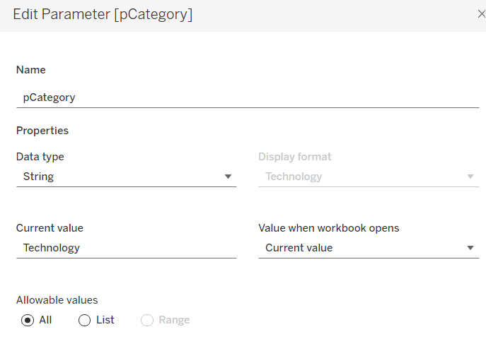
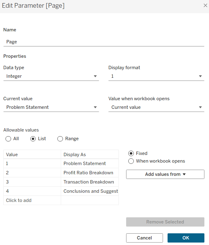
The main crux of this challenge is measure swapping, so for this we need a parameter
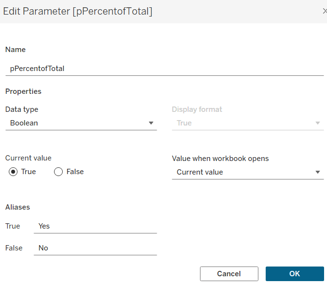
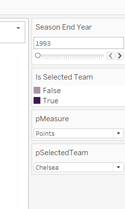
pMeasure
integer parameter listing values 1 to 4 which are aliased as per the screen shot below. Default value is 1 (Points).
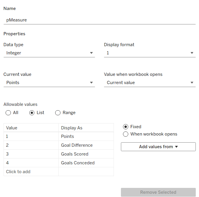
Note – you can use a string parameter with the actual words. I just chose to use this method to demonstrate the aliasing ability. Also when referencing this parameter in a CASE statement (which we’ll do shortly), using integer values for comparisons is slightly more efficient than string comparisons.
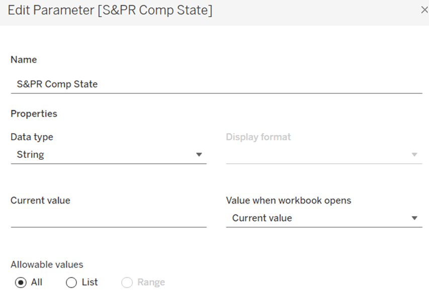
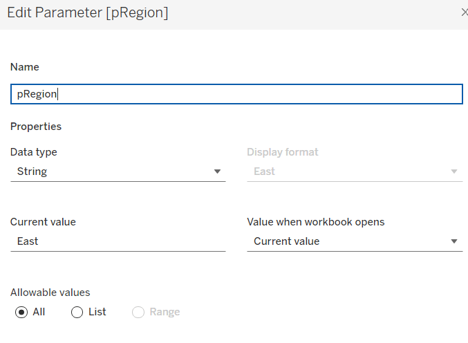
We also need the user to have the ability to select the team they want to track
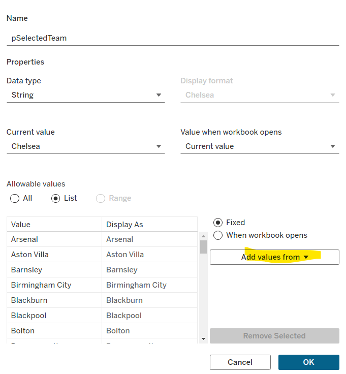
pSelectedTeam
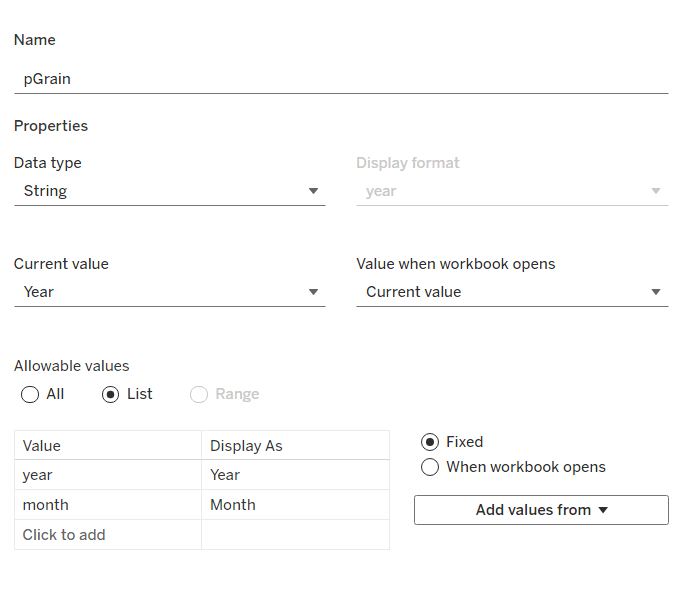
string parameter defaulted to your preferred team (I chose Chelsea). This is a List parameter that is populated from the Team field via the Add values from button
Building the calculations
We need to determine the measure to display based on the parameter selection
Measure to Display
CASE [pMeasure]
WHEN 1 THEN SUM([Cumulative Points])
WHEN 2 THEN SUM([Cumulative Goal Difference])
WHEn 3 THEN SUM([Cumulative Goals For])
WHEN 4 THEN SUM([Cumulative Goals Against])
END
We also will need to colour the bars based on the selected team
Is Selected Team
[Team]=[pSelectedTeam]
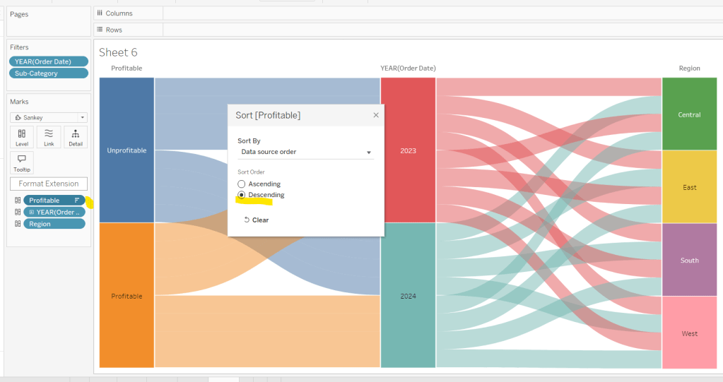
and we need to sort the data based on best to worst, but need to consider that for Goals Conceded, the higher the value the worse the team is.
Sort Measure
IF [pMeasure] = 4 THEN [Measure to Display]*-1 ELSE [Measure to Display] END
We only want to show teams once they start participating in a Season. For this, we need to identify the team’s 1st season in the EFL
1st Season per Team
{FIXED [Team]: MIN(IF [Cumulative Points] > 0 THEN [Season End Year] END)}
and then we can create a field we can filter on, based on this
Show Team
[Season End Year]>=[1st Season per Team]
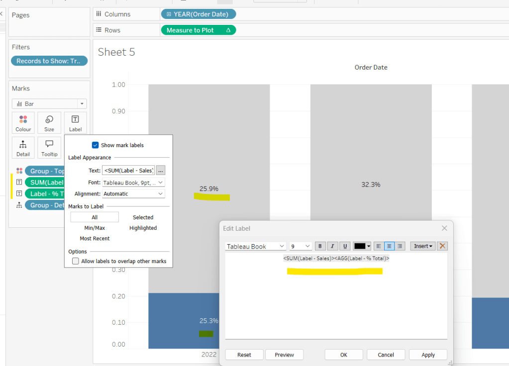
We only want to show a label against the 1st team and the selected team, so create
Label to display
IF MIN([Is Selected Team]) OR FIRST()=0 THEN [Measure to Display] END
and finally, we need to display the value of the current season’s measure on the tooltip, as well as the cumulative value, so we need another case statement
Tootltip Measure
CASE [pMeasure]
WHEN 1 THEN SUM([Points])
WHEN 2 THEN SUM([Goal Difference])
WHEn 3 THEN SUM([Goals For])
WHEN 4 THEN SUM([Goals Against])
END
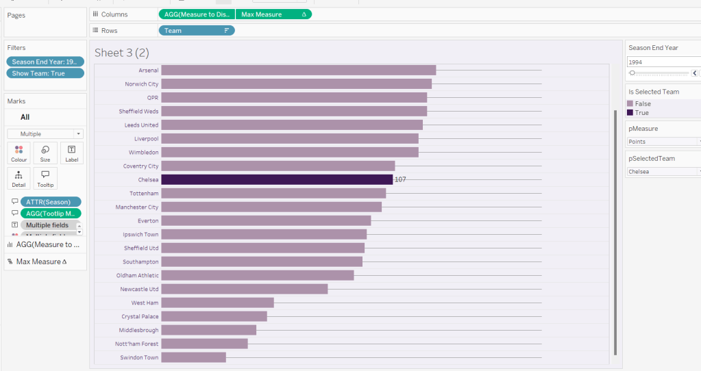
Building the core bar chart
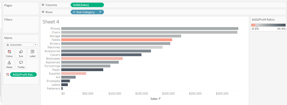
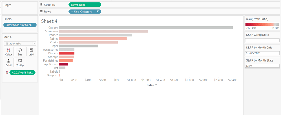
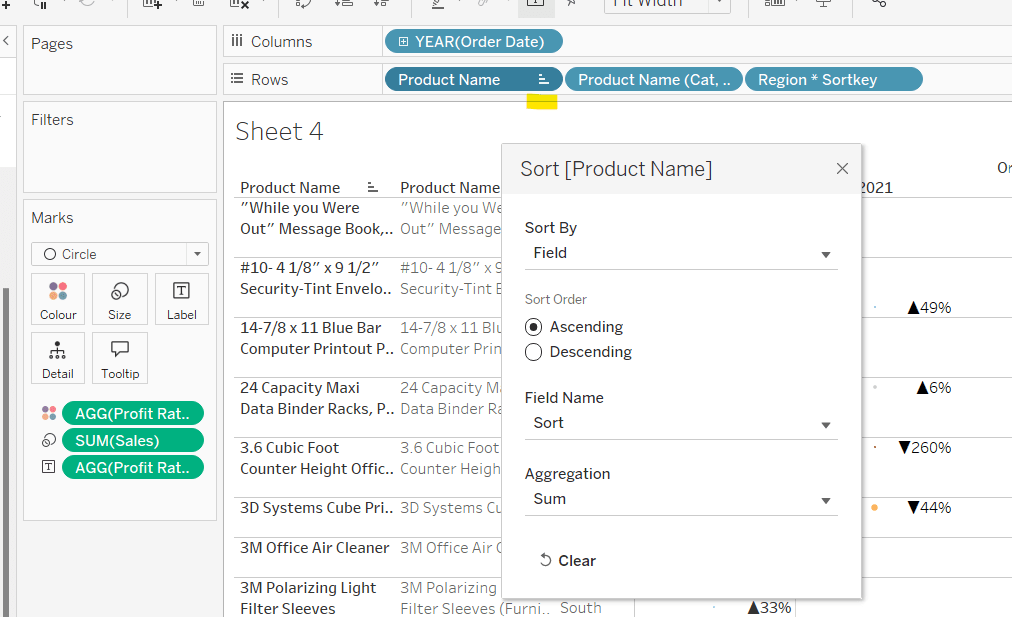
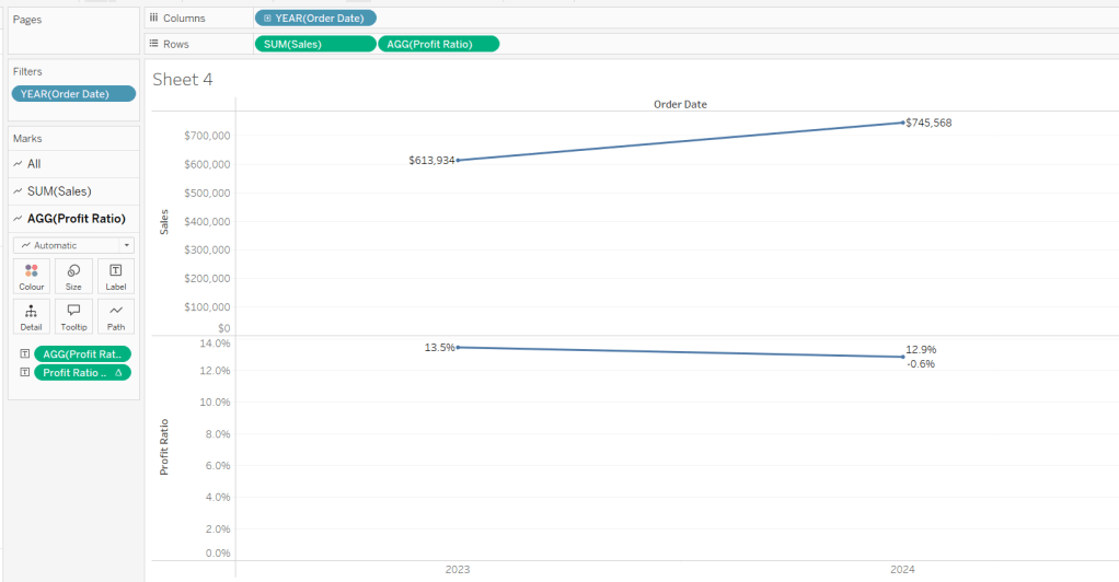
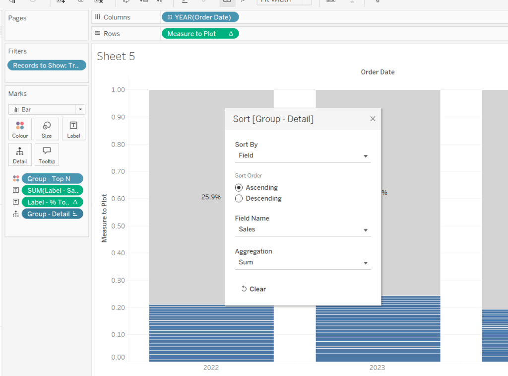
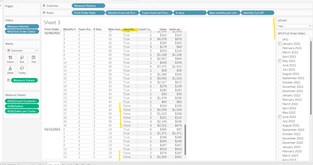
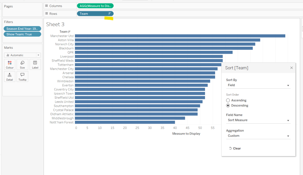
On a new sheet, add Team to Rows and Measure to Display to Columns. Add Season End Year to Filter and select 1993. Add Show Team to Filter and select True. Apply a sort to the Team field to sort by the field Sort Measure descending.
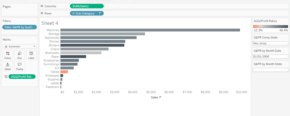
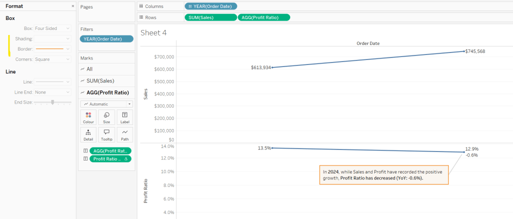
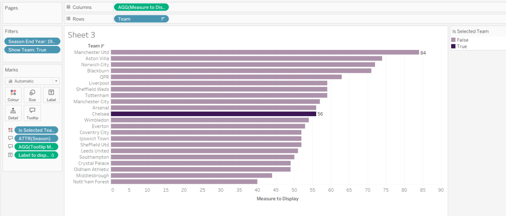
Add Is Selected Team to Colour and adjust accordingly. Add Label to display to Label. Add Season and Tooltip Measure to Tooltip and update accordingly,
Show the pMeasure and pSelectedTeam parameters and the Season End Year Filter. Adjust the Season End Year filter control so that the All option isn’t available and it displays as a single value slider control.
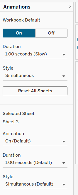
Move the Season End Year filter control on by one value and notice how the chart transitions. Adjust the Animations settings (Format menu > Animations) to be sequential and slow
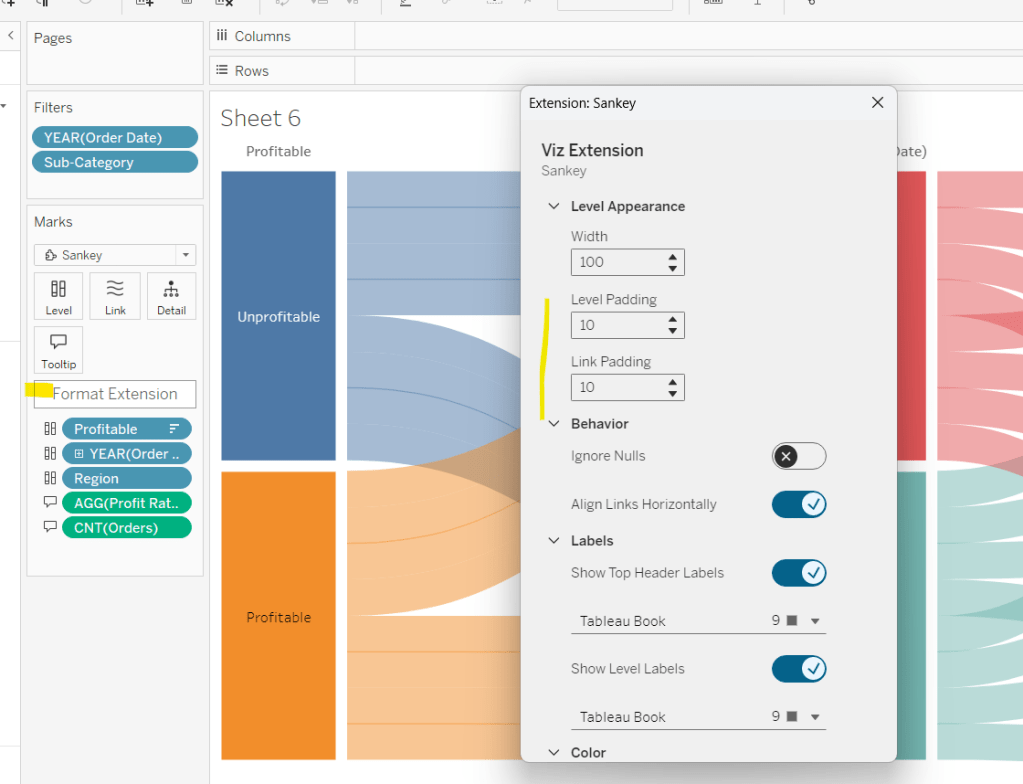
Finally tidy up the display by
- hiding the Measure to Display axis (right click > uncheck show header)
- hiding the Team row label (right click > hide field labels for rows)
- widen each row a bit
- hide gridlines, zero lines, axis rulers and axis ticks
- add pale grey row dividers
- set the background colour of the worksheet
- adjust the font of the row labels – I used Tableau Book 8pt in colour #3e1756 (dark purple)
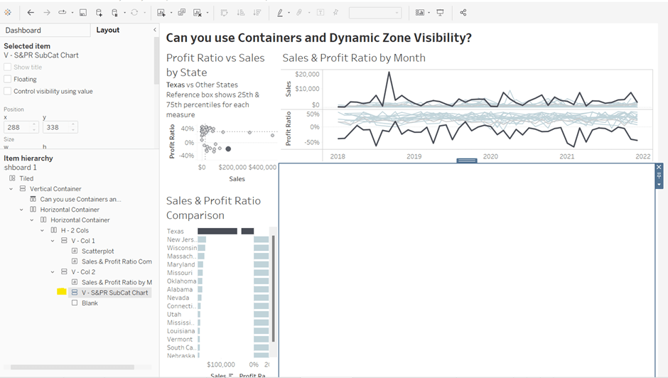
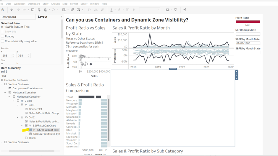
Name the sheet Core or similar and add to a dashboard setting it to Fit Entire View
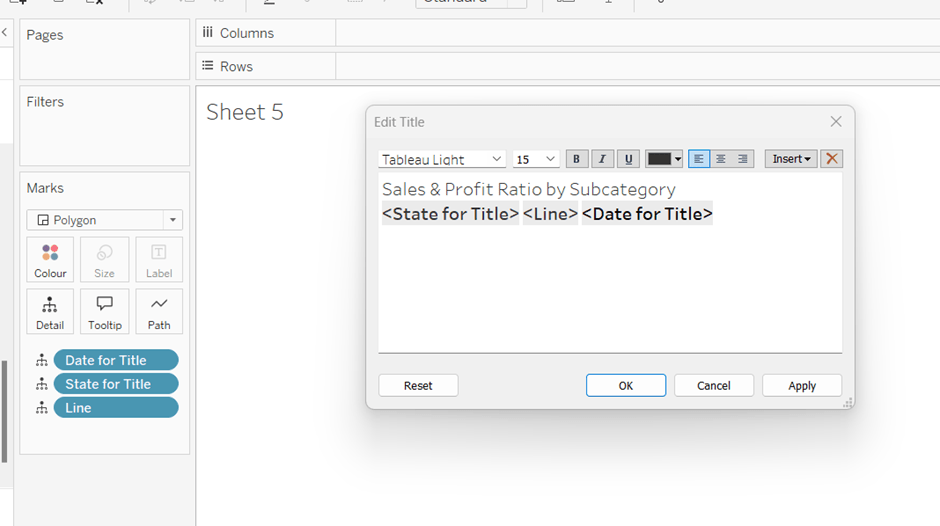
Add a title to the dashboard that references the pSelectedTeam parameter.
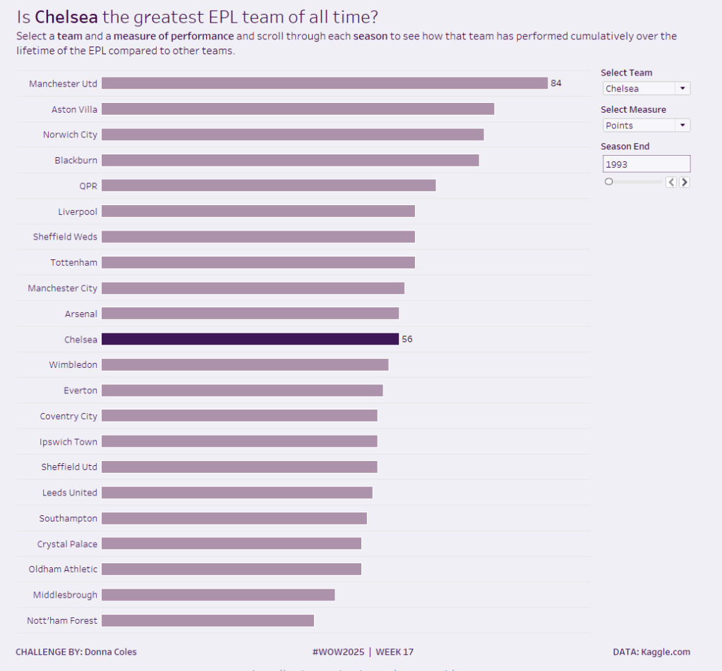
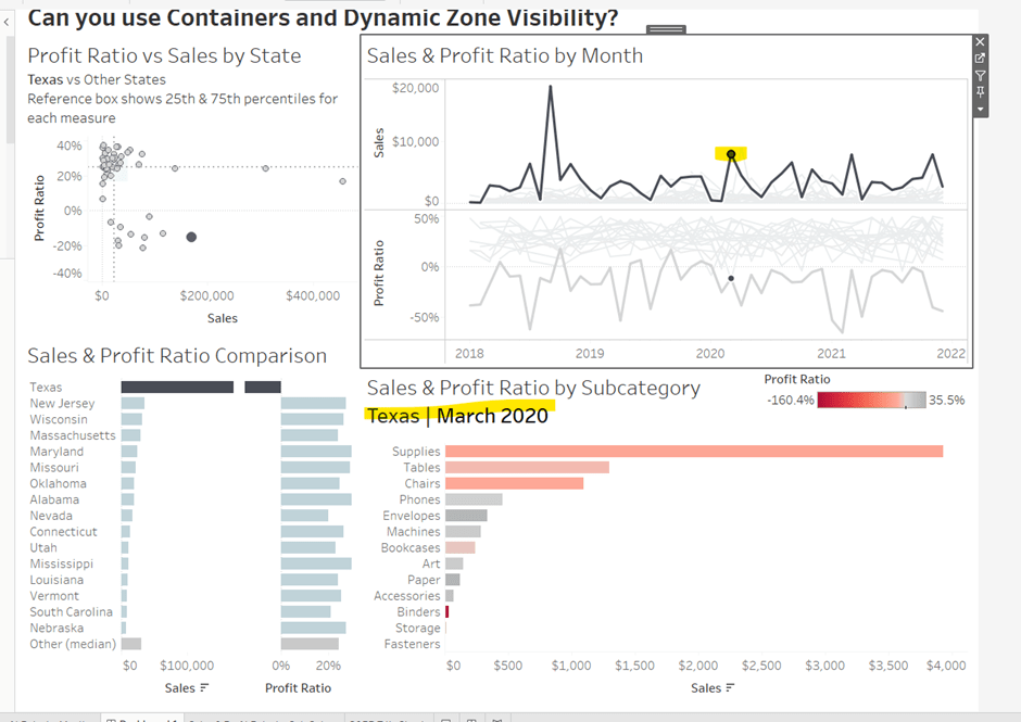
My core viz is here.
Building the bonus viz
Start by duplicating the core viz sheet.
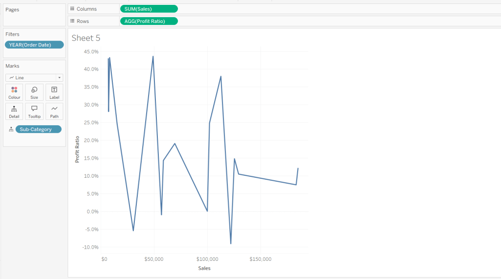
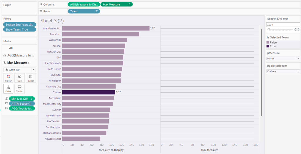
We’re going to use a gantt bar to simulate a central line for each row. This bar needs to extend to the largest measure in the table for every row, so this is the point we’ll plt
Max Measure
WINDOW_MAX([Measure to Display])
Add this to the Columns shelf, and on the Ma Measure markls card that gets added, remove the Is Selected Team from the Colour shelf, and change the mark type to gantt bar.

The bar needs to extend to the 0 or the minimum value in the window (if its less than 0), so we need a field to show the difference between the max and the minimum of 0 or the ‘window min’, but we need to multiple by -1 so the size extends in the right direction.
Max-Min Diff
([Max Measure] – MIN(WINDOW_MIN([Measure to Display]),0)) * -1
Add this to the Size shelf, and then update the size to be as small as possible. Remove Label to Display from the marks card and add a border the same colour as the background to the Gantt bar (via the Colour shelf) to make the line very narrow.
Add Team to the Label shelf and align centre left. Format the label text to be 8pt and dark purple. Then make the chart dual axis and synchronise the axis.
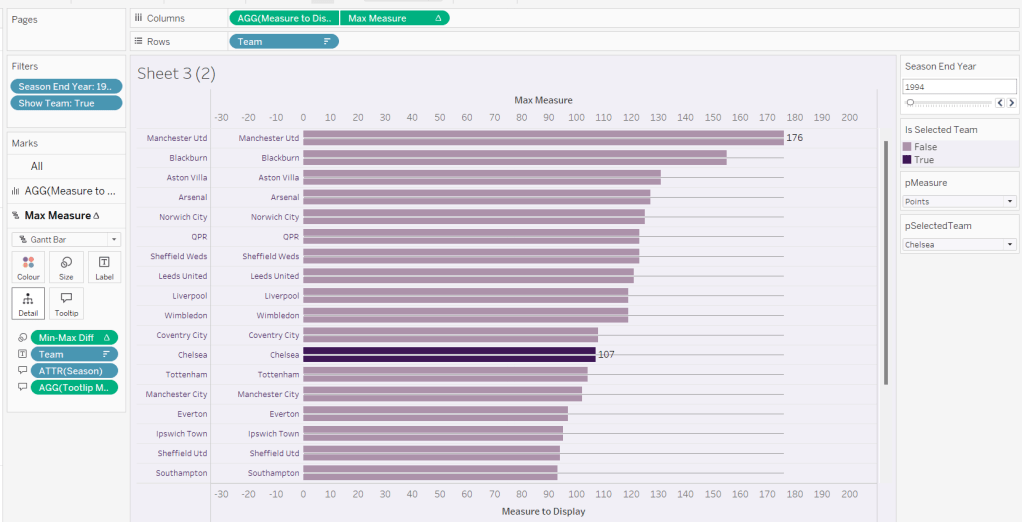
Right click the top axis and select move marks to back. Then hide both axis (right click, uncheck show header) and hide the Team pill on Rows too (again uncheck show header)
Verify the Tooltip on the gantt bar displays the same as on the main bar. If not add the relevant fields and adjust to match.
Tidy up the formatting by removing the row and column dividers. If need be adjust the colour of the Gantt bar to be a paler grey.
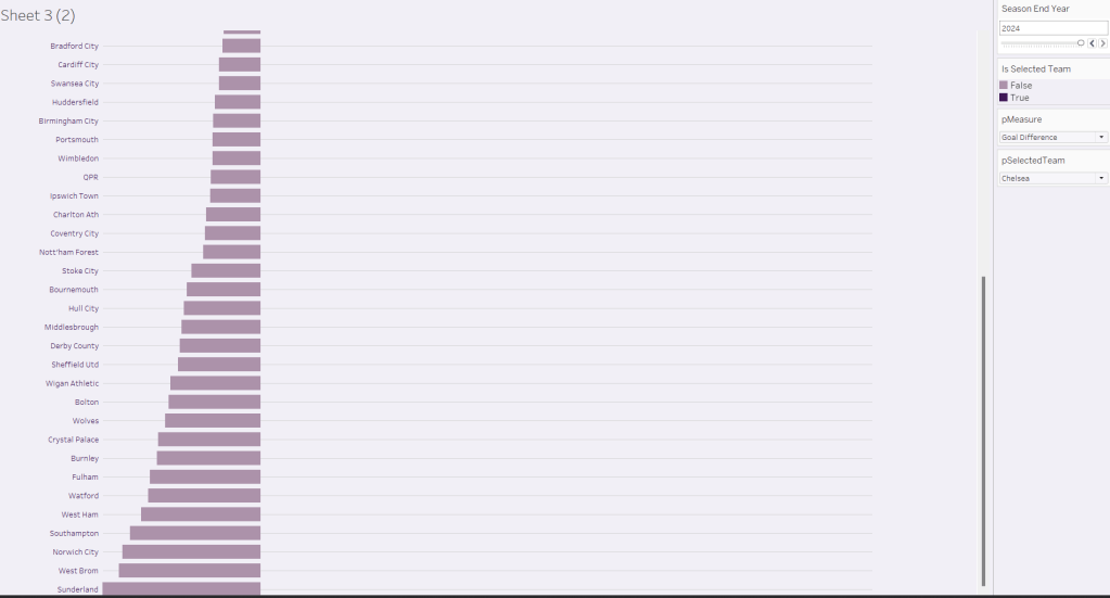
Change the measure value to Goal Difference and adjust the year to 2024 and check the display looks as expected, especially at the bottom – the gap between the label of the team at the bottom and the bar is minimal.
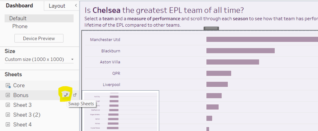
Add the chart to a dashboard – the simplest way is to duplicate the core dashboard and then use the swap sheets feature to quickly swap the main vizzes.
My published viz is here
Happy vizzin’!
Donna