As we’re in the midst of the 33rd Summer Olympics, I set an Olympic-ish themed challenge this week which was a recreation of a Viz built by my Biztory colleague, James Newton (Twitter|X / Linked In).
Whilst fun, I knew this was likely to be a bit tricky, so I tried to provide a lot of pointers, and several hints – hopefully they helped, but obviously this guide should clarify further 🙂
Modelling the data
3 csv data sets were provided, and I advised how they needed to be joined using the physical model rather than using logical relations.
Connect to the points.csv file, then click on the context menu and select Open to ‘open’ the physical layer.

Then add the Records data to the canvas and join as a left join on Lane and Event

Then add in the Scaffold data and join to Points with a left join on the Events field.

Define the parameters
Lanes 5 and 6 will be defined via user inputs, so we need parameters to capture this information
pRunner1
string parameter defaulted to any name (eg Donna)

pRunner2
string parameter defaulted to another name (eg Lorna)

pRunner1Time
string parameter defaulted to a time (in seconds) that it may take the 1st runner to run 100m eg 17.5. Note this is a string parameter as we need to handle a value for when there is no value any numeric value like 0 isn’t going to work in this situation.

pRunner2Time
string parameter defaulted to a time (in seconds) that it may take the 2nd runner to run 100m eg 20

Defining the calculations
Let’s start by adding some data to a table to help validate the calculations we need to build.
From the Points data, add Event and Lane to Rows. Then add X Start, X End, Y Start and Y End to Rows as discrete dimensions (unaggregated blue pills).

As we can see, the X coordinates are the same for each lane, as the race starts and finishes at the same points along the x-axis for every runner. The Y coordinates differ per runner as this reflects the ‘lane’ they’re in, but the values are the same for both the start & end points.
So first off, we want to calculate the ‘distance’ of the race
Start to End Distance
[X End] – [X Start]
Make this a dimension then add to Rows as a discrete (blue) field.

The 330 ‘points’ between the X Start and the X End essentially represent the 100 metres to be ‘run’.
To enable the effect of ‘running’ the 100 metre race, the 100m is split into ‘markers’ where we will plot the position of a runner as it ‘runs’. The number of markers (50) is defined within the Scaffold data, but rather than ‘hardcode’ the value, I calculated the number via
Count Markers
{FIXED: MAX([Marker])}
Doing this, means you can adjust the number of markers in the Scaffold data if you wish. From this, we can then work out how much distance is covered per marker
Distance per Marker
[Start to End Distance]/[Count Markers]
Add this into the table as a discrete dimension.

Next we want to establish the time of the slowest runner, but first we need to get a handle on the times of the runners from the parameters.
Runner 1 Time
IIF([pRunner1Time] = ”, NULL, FLOAT([pRunner1Time]))
Runner 2 Time
IIF([pRunner2Time] = ”, NULL, FLOAT([pRunner2Time]))
As we captured the times as strings in the parameters we can now convert to a numeric float value, and capture a NULL if no data is provided.
Now we can work out the slowest time, which is the maximum of the times provided for lanes 1-4 and the times in the parameters. I’ve managed this in a single calculation
Slowest Time
{FIXED : MAX(MAX([Time], MAX(IFNULL([Runner 1 Time],0), IFNULL([Runner 2 Time],0))))}
Most of the time when we use the MAX() function we are just passing a single expression eg MAX([Sales}) to get the maximum value from the [Sales] field. But you can also use MAX() to compare the maximum values from two expressions eg MAX([Value1], [Value2]) will get all the values stored in both the [Value1] and [Value2] fields and return the overall maximum of both.
So breaking down the expression above, we’re replacing any null values for Runner 1 and 2 with 0, then returning the maximum of these two runners via the inner MAX expression ie
Max of parameters : MAX(IFNULL([Runner 1 Time],0), IFNULL([Runner 2 Time],0))
and then comparing this with the Time of the runners from lanes 1-4
(MAX([Time], <Max of parameters>)
This is all then wrapped in a FIXED Level of Detail calc as we want the value to perpetuate across every row of data. Note, the outer MAX that forms part of the FIXED calc could just as easily be a MIN or AVG.
Add this to the table as a discrete dimension. In this instance the value is 20 as the largest value comes from one of the parameters. You can set these to empty or change the timings to see how the field changes.

Now we compare each runner’s time against the slowest time. Add in Time from the Records data source to the table as a discrete dimension.

Lanes 4 & 5 are Null, so we need to get a field that stores the runner’s time for every lane
Lane Time
IFNULL([Time],
(IF [Lane] = 5 THEN [Runner 1 Time] ELSEIF [Lane] = 6 THEN [Runner 2 Time] END)
)
Use the Time field, but if null, get the relevant time associated to the Lane. Format this to a number with 2dp and add to the table as a discrete dimension.

Next we calculate the proportion of time for each Lane (runner) compared to the slowest runner
Time % of Slowest Time
[Lane Time]/[Slowest Time]
Again add to the table as a discrete dimension

Now, if we assume the slowest runner (in this case Lane 6 at 20s) covers the Distance per Marker (6.6 ‘points’) for every marker in the whole of the ’50 point’ race, then we can assume that faster runners, cover a greater distance for each marker, and that is based on the time proportion calculated above. Eg if a runner took 10s (half the time), we would expect them to cover double the distance (13.2 points) for each marker.
Distance per Marker per Lane
[Distance per Marker] / [Lane Time % of Slowest Time]
Add this to the table too as a discrete dimension. This is essentially a ‘constant’ value per runner

Now we can work out the x-coordinate for each marker. So add Marker from the Scaffold data into the table, so we now have 51 rows per lane, and then create
X to Plot
MIN(([X Start] + ([Marker] * [Distance per Marker per Lane])), [X End])
As we need the runner to stop once they reach the end, we are using the MIN([Value1],[Value2]) functionality again to just return the end position of the race. Add this field to Text.

We can see that for Lane 1, they have reached the end of the race at the 24th marker, and the X to Plot has incremented by 13.78 ‘points’ for each marker. While if you look at Lane 6, the slowest runner, X to Plot increments by 6.6 ‘points’ and reaches the end on the last marker.
We now have the core of the data we need to build the viz.
Creating the race
On a new sheet, add X to Plot as a continuous dimension (green unaggregated pill) to Columns and Y Start to Rows (also as a continuous dimension)

Change the mark type to shape and assign the custom runner shape (see here for info on how to do this). Add Lane to Colour and adjust accordinglt. Increase the Size a bit.

Add the background image (Maps > Background Images > <Datasource Name> > Add Image). Browse to the image file you should have saved and then adjust the values to reflect the size of the image (500 wide by 288 high), so X field that references X to Plot goes from 0 to 500, and the Y Field that references Y Start goes from 0 to 288.

Then fix the X to Plot axis to range from 0 to 500,and the Y Start axis from 0 to 288.

This should make the runners appear to be in each lane.
Add Marker to the Pages shelf. The page control should display starting at 0 and only 1 runner image per lane should display. Adjust the Size of each runner if need be.

Press the ‘play’ button on the control, and set the speed to max and you should see the runners move down the track.
Labelling the viz
We need to get the name of runner in each lane, which is sourced either from the parameters for lanes 5 & 6 or from the Records data, BUT we only want the label to display at the start or end of the race.
Label – Runner
IF [Marker] = 0 THEN
IF [Lane] = 5 THEN [pRunner1]
ELSEIF [Lane] = 6 THEN [pRunner2]
ELSE [Record (Records.csv1)] + ” ” + [Gender (Records.csv1)]
END
ELSEIF [Marker] = [Count Markers] THEN
IF [Lane] = 5 THEN [pRunner1]
ELSEIF [Lane] = 6 THEN [pRunner2]
ELSE [Record (Records.csv1)] + ” ” + [Gender (Records.csv1)]
END
END
We also want the runner’s Time to display on the label, but only at the end of the race
Label – Time
IF [Marker] = [Count Markers] THEN [Lane Time] END
Format this to a number with 2 dp and suffixed with ‘s’
Add both these fields to the Label shelf and arrange accordingly. Set the font to match mark colour and align label middle left.. Test the labels display as expected by setting the marker value back to 0 and playing the race through again.

Adding Tooltips
Create the field
Tooltip – Athlete
IF [Lane] = 5 THEN [pRunner1]
ELSEIF [Lane] = 6 THEN [pRunner2]
ELSE [Athlete (Records.csv1)]
END
Then add this field, Lane Time, Gender and Record to the Tooltip shelf and adjust accordingly.
Tidying up
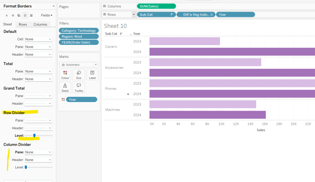
Finally remove all gridlines, zero lines, axis rulers & ticks, row/column dividers and hide the axes.
Add the sheet to a dashboard and arrange the objects as required, using containers to help organise the parameters and controls, and setting a background colour to some objects when required.
Customise the page control object so it only shows the slider and playback controls. Unfortunately, when you publish to Tableau Public, the speed controls won’t display, so the runners won’t ‘run’ as fast on Public 😦
My published viz is here. I hope you enjoyed it, and didn’t find it too complicated!
Happy vizzin’!
Donna