Let’s Practice RegEx in Tableau with Generative AI

Yoshi set this week’s challenge which focused on 2 areas : the use of tools such as CHAT GPT to help us create Tableau RegEx functions (which are always tricksy), and the build of the chart itself.

Creating the REGEX calculated fields

I chose to use CHATGPT and simply entered a prompt as

“give me a regex expression to use in Tableau which extracts a string from another string in a set format. The string to interrogate is”

and then I pasted in the string I’d copied from one of the Session Html fields. I got the following response

along with many more code snippet examples. I used these to create

Session Title

REGEXP_EXTRACT([Session Html], '<div class="title-text">(.*?)</div>')

Description

REGEXP_EXTRACT([Session Html], '<div class="description"[^>]*><div>(.*?)</div>')

Location

REGEXP_EXTRACT([Session Html], '<span class="session-location"[^>]*>(.*?)</span>')

Session Level

REGEXP_EXTRACT([Session Html], 'session-level-([a-zA-Z]+)')

Alias this field to show the values in proper case (ie ‘Advanced’ rather than ‘advanced’) and display Null as ‘All Levels’

Session Date

REGEXP_EXTRACT([Session Html], '<span class="semibold session-date">(.*?)</span>')

Session Time

REGEXP_EXTRACT([Session Html], '<span class="semibold session-time">(.*?)</span>')

Start Time

REGEXP_EXTRACT([Session Html], '<span class="semibold session-time">([0-9: ]+[AP]M)')

End Time

REGEXP_EXTRACT([Session Html], '- ([0-9: ]+[AP]M)')

Creating the additional fields

All of the RegEx functions return string fields. To build the viz, we need actual date fields and additional information

AM|PM

IIF(CONTAINS([Start Time],’AM’), ‘AM’, ‘PM’)

Date

DATE(DATEPARSE(“MMMM d yyyy”, SPLIT([Session Date], “, “, 2) + ” 2023″))

returns the day of the session as a proper date field, all hardcoded to 2023, since this is when the data is from.

Start Date

DATETIME(STR([Date]) + ” ” + [Start Time])

returns the actual day & start time as a proper datetime field.

End Date

DATETIME(STR([Date]) + ” ” + [End Time])

Duration

DATEDIFF(‘second’, [Start Date], [End Date])

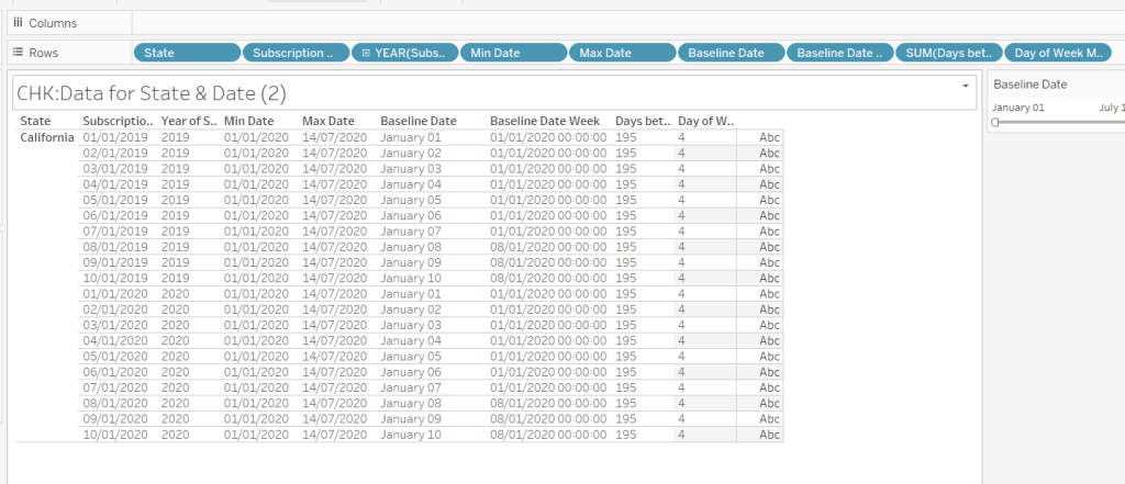
Add fields to a table as below

Firstly, when we build the viz, we’ll need to sort it based on the Start Date, the Session Level (where Advanced is listed first, and All Levels last) and the Duration (where longer sessions take higher precedence) . For this we need a new field which is a combination of information related to all these values.

Sort

STR([Start Date]) + ‘ – ‘ + STR(
CASE [Session Level]
WHEN ‘advanced’ THEN 4
WHEN ‘intermediate’ THEN 3
WHEN ‘beginner’ THEN 2
ELSE 1
END
) + STR([Duration]/100000)

(this just took some trial and error)

Add this to the table after the Session ID pill and then apply a Sort to the Session ID pill so it is sorting by the Minimum value of the field Sort Ascending. You should see that when the start time and session level match, the sessions are sorted with the higher duration first.

The viz also lists the AM & PM sessions as separate instances, where the 1st session of the PM session is displayed on the same ‘row’ as the 1st session of the AM session. To handle this we need

Session Index

INDEX()

Make this discrete and add to the table after the AM|PM pill. Change the table calculation so it is computing by all fields except AM|PM and Session Date. The numbering should restart at each am/pm timeslot

Finally, the last field we need to build this viz, is another date field, so we can position the gantt chart bars in the right places. As the viz already segments the chart by Session Date and AM|PM, we can’t reuse the existing Start Date field as this will display the information as if staggered across the 3 days. Instead we want to create a date field, where the day is the same for al the sessions, but just the time differs

Baseline Date

DATETIME(STR(#2023-01-01#) + ” ” + [Start Time])

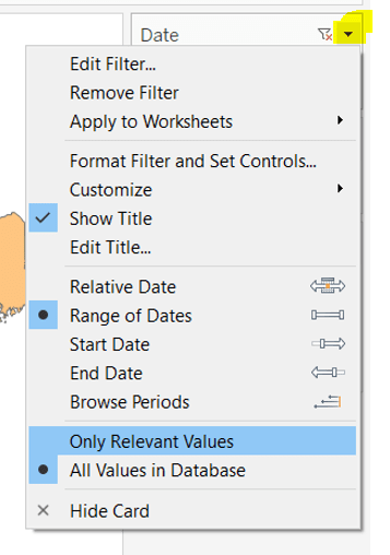
the date 01 Jan 2023 is arbitrary and could be set to any day. Add this into the table, so you can see what it’s doing. You will probably need to adjust the table calculation on Session Index again to include Baseline Date in the list of checked fields.
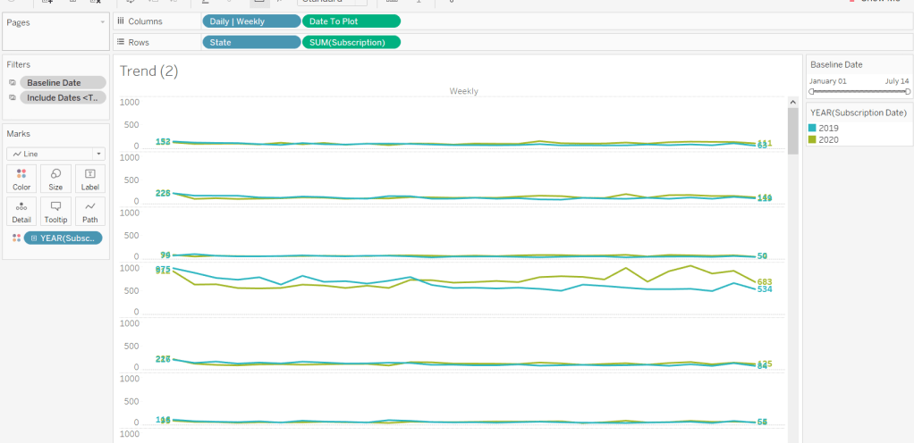
Building the viz

On a new sheet, add Session Date to Columns and manually re-order so Tuesday listed first. Then add AM|PM to Columns . Add Baseline Date as a continuous exact date (green pill) to Columns . Add Session Id to Detail then add Session Index to Rows and adjust the table calculation so it is computing by all fields except Session Date and AM|PM.

Create a new field

Size

SUM([Duration])/86400

and add this to the Size shelf. 86400 is the number of seconds in 24hrs, so adjusts the size of the gantt bars to fit the timeframe we’re displaying.

Add Session Level to Colour and adjust accordingly. You will need to readjust the Session Index table calc to include Session Level in the checked fields. Add a border to the bars. Edit the Baseline Date axis so the axis ranges are independent

Add Description and Session Title to Detail and again adjust the Session Index table calc to include these fields too. Apply a Sort to the Session Id field so the data is sorted by the Sort field descending

Add Location, Start Time and End Time to Tooltip, and update accordingly. Then apply formatting to

  • change font of the Session Date and AM|PM header values
  • remove the Session Date/ AM|PM column heading label (right click > hide field labels for columns)
  • Hide the Session Index field
  • Hide the Baseline Date axis
  • Add column banding so the Wednesday pane is coloured differently

Add the ability to highlight the Session Title and Description by selecting Show Highlighter from the context menu of each pill

Then add the sheet to a dashboard, using containers to display the colour legend and the highlighter fields.

And that should be it. My published viz is here.

Happy vizzin’!

Donna

Can you show YTD and PYTD, whilst also being able to change the date range and switch between Month & Week?

It was Lorna’s turn to set the challenge this week – to compare YTD with Previous YTD while also filtering date ranges which updated based on the year of focus. She hinted it was a great use case for an INCLUDE LoD and I have to admit that seemed to fry my brain! I spent a couple of hours trying various concepts and then put it to bed as I wasn’t progressing.

When Rosario Gauna published her solution, I had a quick look and realised that there was no need for an LOD after all, and I shouldn’t have got hung up on the hint. So thanks Rosario!

Setting up the data

The data set provided contains 4 complete years worth of data from 1st Jan 2021 to 31st Dec 2024. In order to simulate ‘YTD’ for 2024 and ensure my workbook would always show the concept of a partial year, I created a parameter

pToday

date parameter defaulted to 3 July 2024

and then I created

Records to Keep

[Order Date]<= [pToday]

In a typical business scenario, the pToday parameter would simply be replaced by the TODAY() function.

I then added this as a data source filter (right click data source > add data source filter) and set to True to restrict the data from 01 Jan 2021 through to 03 July 2024.

Setting up the calculations

Before building the Viz, we’re going to work through what calculations are needed to drive the behaviour we require. We’ll do this in a tabular view. First up we will need a couple of parameters

pYear

integer parameter defaulted to 2024 containing a list of values from 2021 to 2024. The display value should be formatted to a whole number without the , separators.

pDatePart

string parameter defaulted to Month containing a list of 2 values Month and Week.

Show these parameters on a sheet.

On the sheet, add Order Date as a discrete exact date (blue pill) to Rows.

The first thing we will do is identify the set of Order Dates that we need to consider based on the pYear parameter. That is if pYear is 2024, we want to consider the Order Dates in 2024 and the Order Dates in 2023. But if the pYear is 2023, we want to consider all Order Dates in 2023 and 2022. When we do identify these dates, we will ‘baseline’ them to all align to the focus year (ie the pYear value).

Date Baseline

DATE(IF YEAR([Order Date]) = [pYear] THEN [Order Date]
ELSEIF YEAR([Order Date]) = [pYear]-1 THEN DATEADD(‘year’, 1, [Order Date])
ELSE NULL
END)

Add this as a discrete exact date (blue pill) to Rows.

If you scroll through, you should see how the Date Baseline field is behaving as you change the pYear value.

Now we only want to include rows with dates, and in the case of 2024 v 2023, we only want dates up to ‘today’.

Filter Dates

IF [pYear] = YEAR([pToday]) THEN
[Date Baseline] <= [pToday]
ELSE
[Date Baseline] <= MAKEDATE([pYear], 12, 31)
END

If the pYear parameter matches the year of ‘Today’, then only include dates up to ‘Today’, otherwise include dates up to 31 Dec of the selected year.

Add this to the Filter shelf and set to True.

When pYear is 2024, you can see that we have Order Dates from 01 Jan 2023 to 03 Jul 2023 and then 01 Jan 2024 to 03 Jul 2024. But changing pYear to 2023, you get all dates through from 01 Jan 2022 to 31 Dec 2023.

Add Date Baseline to the Filter shelf, and select Range of Dates, then choose the Special tab and verify All dates is selected and select Apply to commit this option.

Show the Date Baseline filter to display the range control filter.

Changing the pYear parameter will change the start & end dates in the Date Baseline filter to match the year selected. But with 2024 selected, the range ends at 31 Dec 2024. We don’t want this – we only have data up to 3rd July 2024. To resolve this, set the property of the filter control to Only Relevant Values

Adjust the date ranges and the records in the table should adjust too. If you change the pYear parameter after you’ve adjusted the date range, you’ll need to reset/clear the date range filter.

The next thing we need to handle is the switch between months and weeks. For this create

Date to Display

DATE(CASE [pDatePart]
WHEN ‘month’ THEN DATETRUNC(‘month’,[Date Baseline])
ELSE DATETRUNC(‘week’, [Date Baseline])
END)

Add this as a discrete exact date to Rows and you can see how this field works when the pDatePart field is altered.

So now we have the core filtering functionality working, we need to get the measures we need

YTD Sales

IF YEAR([Order Date]) = [pYear] THEN [Sales] END

PYTD Sales

IF YEAR([Order Date]) = [pYear]-1 THEN [Sales] END

format both of these to $ with 0 dp

% Diff

(SUM([YTD Sales]) – SUM([PYTD Sales]))/SUM([PYTD Sales])

custom format this to â–²0%;â–¼0%;0%

Building the KPI

On a new sheet, double click into Columns and type MIN(0), then repeat, so there are 2 instances on MIN(0) on Columns and 2 marks cards.

Change the mark type on the All marks card to shape, and select a transparent shape (see here for details). Set the sheet to Entire View.

On the 1st MIN(0) marks card, add YTD Sales to Label. Then adjust the label font and text and align middle centre.

On the 2nd MIN(0) add PYTD Sales and % Diff to Label and adjust the layout and formatting as required. Align middle centre.

On the tabular worksheet we were using to test things out, set both the filters to ‘apply to worksheets > all using this data source’, so persist the changes made on one sheet to all others.

On the All marks card, add Date Baseline to Tooltip and adjust to use the MIN aggregation. Then add another instance of Date Baseline to Tooltip and adjust to use the MAX aggregation. Update the Tooltip accordingly.

Remove all row/column dividers, gridlines, zero lines. Hide the axis. Name the sheet KPI or similar.

Building the line chart

ON a new sheet add Date to Display as a continuous exact date (green pill) to Columns and YTD Sales to Rows. Show the pYear and pDatePart parameters. The Date Baseline and Filter Date fields should have automatically been added to the Filter shelf. Show the Date Baseline filter.

Drag the PTYD Sales field from the data pane onto the YTD Sales axis and drop it when the cursor changes to a double green column icon.

This will automatically adjust the pills to include Measure Names and Measure Values onto the view. Adjust the colours of the lines and ensure the YTD Sales line is displayed on top of the PYTD Sales line (just reorder the values in the colour legend if need be).

Add YTD Sales and PYTD Sales to Tooltip and adjust accordingly. Edit the Value axis and adjust the title of the axis to Sales. Remove the title from the Date to Display axis.

Building the dashboard

Use a combination of layout containers to add the objects onto a dashboard. I started with a horizontal container, with a vertical container in each side.

My published viz is here.

Happy vizzin’!

Donna

Antarctic Ice Extent

It was Luke’s turn to set the #WOW2023 challenge this week and he chose to focus on remaking a visualisation relating to the change in the Antarctic Sea Ice, inspired by charts created by Zach Labe.

The challenge involved the use of extensive calculations, which at times I found hard to validate due to the steps involved in reaching the final number, and only having visibility of the final number on hover on a point on the chart. If it didn’t match, it became a bit of a puzzle to figure out where in the process I’d gone wrong.

Getting the data for the faded yearly line charts was ok, but I ended up overthinking how the decade level darker line chart was calculating and couldn’t get matches. Anyway, after sleeping on it, I realised my error, and found I didn’t need half the calculations I’d been playing with.

So let’s step through this. As we’re working with moving averages, we’re looking at using table calculations, so the starting point is to build out the data and the calculations required into a tabular form first.

Setting up the calculations

I used the data stored in the Google sheet that was linked to in the challenge, which I saved down as a csv file. After connecting to the file, I had separate fields for Day, Month and Year which I changed to be discrete fields (right click on field and Convert to discrete).

We need to create two date fields from these fields. Firstly

Actual Date

MAKEDATE([Year],[Month],[Day])

basically combines the 3 separate fields into a proper date field. I formatted this to “14 March 2001” format.

Secondly, we’ll be plotting the data on an axis to span a single year. We can’t use the Actual Date field for that as it will generate an axis that runs from the earliest date to the latest. Instead we need a date field that is ‘normalised’ across a single year

Date Normalise

MAKEDATE({max([Year])}, [Month], [Day])

the {max([Year])} notation is a short cut for {FIXED: MAX([Year])} which is a level of detail (LoD) expression which returns the greatest value of the Year field in the data set. In this case it returns 2023. So the Date Normalise field only contains date for the year 2023. Ie if the Actual Date is 01 Jan 2018 or the Actual Date is 01 Jan 2020, the equivalent Date Normalise for both records will be 01 Jan 2023.

Let’s start to put some of this out into a table.

Put Year on Columns, and Date Normalise as a blue (discrete) exact date field on Rows. Add Area(10E6M2) to Text and change to be Average rather than Sum (in leap years, the 29 Feb seems to have been mapped to 01 March, so there are multiple entries for 01 March). This gives us the Area of the Ice for each date in each year.

We need to calculate the 7 day moving average of this value. The easiest was to do this is add a Moving Average Quick Table Calculation to the pill on the Text shelf.

Once done, edit the table calculation, and set so that is average across the previous 6 entries (including itself means 7 entries in total) and it computes down the table (or explicitly set to compute by Date Normalise).

It is best to create an explicit instance of this field, so if you click on the field and press ctrl while you drag and drop it into the data pane on the left hand side, you can then rename the field. I named mine

Moving Avg: Area

WINDOW_AVG(AVG([Area (10E6M2)]), -6, 0)

It should contain the above syntax as that’s what the table calculation automatically generates. If you’re struggling, just create manually and then add this into the table instead.

Add Area (10E6M2) back into the table too. You should have the below, and you should be able to validate the moving average is behaving as expected

Now we need to work out the data related to the ‘global’ average which is the average for all years across a single date.

Average for Date

{FIXED [Date Normalise]: AVG([Area (10E6M2)])}

for each Date Normalise value. return the average area.

Pop this into the table, and you should see that you have the same value for every year across each row.

We can then create a moving average off of this value, by repeating similar steps above. In this instance you should end up with

Moving Avg Date

WINDOW_AVG(SUM([Average For Date]), -6, 0)

Add into the table, and ensure the table calculation is computing by Date Normalise and again you should be able to validate the moving average is behaving as expected

Note – you can also filter out Years 1978 & 1979 as they’re not displayed in the charts

So now we have the moving average per date, and the global moving average, we can compute the delta

Ice Extent vs Normal

[Moving Avg: Area] -[Moving Avg Date]

Format this to 3 dp and add to the table. You should be able to do some spot check validation against the solution by hovering over some of the points on the faded lines and comparing to the equivalent date for the year in the table.

This is the data that will be used to plot the faded lines. For the bolder lines, we need

Decade

IF [Year] = {max([Year])} THEN STR([Year])
ELSE
STR((FLOOR([Year]/10))*10) + ‘s’
END

and we don’t need any further calculations. To verify, simply duplicate the above sheet, and then replace the Year field on Columns with the Decade field. You should have the same values in the 2023 section as on the previous sheet, and you should be able to reconcile some of the values for each decade against marks on the thicker lines.

Basically, the ‘global’ values to compare the decade averages against are based on the average across each individual year, and not some aggregation of aggregated data (this is where I was overthinking things too much).

Building the viz

On a new sheet add Date Normalise as a green continuous exact date field to Columns, and Ice Extent vs Normal to Rows. Add Year to Detail and Decade to Colour. Adjust colours to suit and reduce to 30% opacity. Reduce the size to as small as possible. Add Decade to Filter and exclude 1970s. Ensure both the table calculations referenced within the Ice Extent vs Normal field are computing by Date Normalise only.

Add Actual Date to the Tooltip and and adjust the tooltip to display the date and the Ice Extent vs Normal field in MSM.

Now add a second instance of Ice Extent vs Normal to Rows. On the 2nd marks card that is created, remove Year from Detail and Actual Date from Tooltip. Increase the opacity back up to 100% and increase the Size of the line. Sort the colour legend to be data source order descending to ensure the lines for the more recent decades sit ‘on top’ of the earlier ones.

Modify the format of the Date Normalise field to be dd mmmm (ie no year). Adjust the Tooltip as below

Make the chart dual axis and synchronise the axis. Remove the right hand axis.

Edit the axis titles, remove row and column dividers and add row & column gridlines.

Adding the labels

We want the final point for date 18 June 2023 to be labelled with the actual Area of ice on that date and the difference compared to the average of that date (not the moving average). I create multiple calculated fields for this label, using conditional logic to ensure the value only returns for the maximum date in the data

Max Date

{max([Actual Date])}

Label:Date

IF MIN([Decade])=’2023′ AND MIN([Actual Date])=MIN([Max Date]) THEN MIN([Max Date]) END

Label: Area

IF MIN([Decade])=’2023′ AND MIN([Actual Date])=MIN([Max Date]) THEN AVG([Area (10E6M2)]) END

Label:Ice Extent v Avg for Date

IF MIN([Decade])=’2023′ AND MIN([Actual Date])=MIN([Max Date]) THEN AVG([Area (10E6M2)]) – SUM([Average For Date]) END

Label:unit of measure

IF MIN([Decade])=’2023′ AND MIN([Actual Date])=MIN([Max Date]) THEN ‘MSM’ END

Label: unit of measure v avg

IF MIN([Decade])=’2023′ AND MIN([Actual Date])=MIN([Max Date]) THEN ‘MSM vs. avg’ END

All these fields were then added to the Text shelf of the 2nd marks card and arranged as below, formattign each field accordingly

And this sheet can then be added to the dashboard. The legend needs be adjusted to arrange the items in a single row.

My published viz is here.

Happy vizzin’!

Donna

Can you do YoY comparisons?

Community month for the #WOW2022 team continued this week, with Liam Huffman setting this challenge to build a year on year comparison chart with twist.

Typically when building YoY charts you compare the month from last year with the same month this year, or a week from last year with this year (eg week 3 2021 v week 3 2022), or a specific date last year with this year (eg 4th March 2021 with 4th March 2022). However for this challenge, the focus was on being able to compare based on equivalent weekdays (at least that’s what I understood from reading). By this I mean if 10 October 2022 is a Monday, that needs to be compared with the equivalent weekday in the previous year. 10 October 2021 was a Sunday, so we actually need to compare Monday 10 Oct 2022 with Monday 11 Oct 2021.

So that’s the direction I took with this challenge, but in doing so couldn’t get the numbers to exactly match with Liam’s solution. Unfortunately I just couldn’t get my head around Liam’s approach even after looking at it. So I’m blogging this based on my interpretation of the requirement, which may be flawed.

Baselining the Dates

When building YoY charts like this which need to be flexible based on the date part selected, you need to ‘baseline’ the dates; well that’s the term I use, others might refer to it as normalising. Ultimately you need to get the dates that span multiple years to all align to the same year, so you have a single x-axis that just spans a single year.

Now based on what I talked about above, its not just a case of changing the year of every Order Date to match for all the records, we need to find the equivalent weekday from the previous year and align that.

To do this I first created a parameter

pToday

date parameter defaulted to 10 Oct 2022

This is simply to provide a constant end point. In a business scenario when the data changes, any reference to pToday would just use TODAY().

I then created

1st Day of Current Year

DATE(DATETRUNC(‘year’, [pToday]))

This returns 1st Jan 2002

I then worked out what weekday this was

Weekday of 1st Day Current Year

//determine the day of the week this year started on, based on todays date
DATENAME(‘weekday’, [1st Day of Current Year])

This returns Saturday

I then wanted to find the date of the first Saturday in every year, but firstly I needed to determine the weekday for each Order Date

Weekday

DATENAME(‘weekday’, [Order Date])

Date of 1st weekday Per Year

//get the first date in each year which falls on the same weekday as the first day of the current year
//ie 1st Jan 2022 is a Saturday. This is day 0 for 2022. We need to find day 0 for every other
//year, which is the date of the first Saturday in that year

{FIXED YEAR([Order Date]): MIN(IF [Weekday]=[Weekday of 1st Day Current Year] THEN [Order Date] END)}

For each year, get all the dates which fall on a Saturday, then returned the earliest one of those.

Popping all this information out in a table, we can see that in 2019, the first Saturday in the year was 5th Jan 2019, so all the records for dates in 2019 are stamped with 5th Jan 2019.

This Date of 1st weekday Per Year is essentially day 0 for each year. We now need to record a number against each day in the year

Days From Date

//get the number of days from the date of 1st weekday per year
DATEDIFF(‘day’, [Date of 1st weekday Per Year], [Order Date])

And with this number, we can now record the equivalent date in 2022 against each date

Baseline Date

//need to normalise all dates for every year to the current year,
//ie Day 0 for every year = 01 Jan 2022

DATE(DATEADD(‘day’, [Days from Date], [1st Day of Current Year]))

Add these fields into the tabular view and you should hopefully see how this is working

Building the Line Chart

We need some additional parameters to help build the chart.

pDatePart

string parameter defaulted to Month, with 3 values listed as shown below

pStartDate

date parameter set to use the 1st Day of Current Year when the workbook opened, meaning current value was 1st Jan 2022

pEndDate

date parameter set to use the pToday parameter when the workbook opened, meaning current value was 10th Oct 2022

With the pDatePart field, we need to define the actual date we’re going to plot

Date to Plot

DATE(DATETRUNC([pDatePart], [Baseline Date]))

when this is set to week, the date for all days in the same week are set to the first date in the week. Similarly, when this is set to month, all dates in the same month are set to 1st of the month.

The data also needs to be filtered based on the start & end dates selected, so we need

Dates to Include

[Baseline Date]>= [pStartDate] AND [Baseline Date]<=[pEndDate]

Add this to the Filter shelf of the tabular view and set to True. Also add Date to Plot into the table, and show all the parameters. Change the dates and the date part field and familiarise yourself with how the parameters impact the data.

Now we’re happy we’ve got all the key fields we need, then create a new sheet, show the parameters and add Dates to Include = True to Filter.

Then add Date To Plot as an exact date continuous (green) pill to Columns and Sales to Rows.

Create

Order Date Year

YEAR([Order Date])

and add to Colour. Adjust the colours accordingly.

Format the Sales axis, so the numbers are displayed as numbers rolled up to thousands (k) with 0 dp. Edit the Date to Plot axis to remove the title, then format the dates displayed to be in dd mmm custom format. Remove all gridlines and zero lines. Only axis lines should be displayed. Update the title.

Add Date to Plot to Tooltip as a discrete attribute (blue pill). Add MIN(Order Date) to Tooltip too. Adjust tooltip wording to suit.

Building the bar chart

Add Order Date Year to Rows and Sales to Columns. Sort Order Date Year descending.

Add Order Date Year to Colour. Adjust the opacity to about 50% and add a border. Widen the rows. Add Sales to Label and format label to be $K to 1 dp.

Add another instance of Sales to Detail, then adjust to use a Quick Table Calculation of Percent Difference. Move this pill from Detail to Label. Adjust the table calculation so it is relative to Next rather than previous

Format the Sales field that has the table calc, so it is custom formatted to ↑ 0.0%; ↓ 0.0%

Modify the label so the % change is in ( ) .

Add MIN(0) to Columns (type directly in to the columns shelf). Remove the two Sales fields from the marks card, and add another instance of Order Date Year to the Label shelf. Adjust the Label so the font is larger, matches mark colour and is rotated.

Make the chart dual axis, and synchronise axis.

Turn off all tooltips, hide the Order Date Year column and both axis. Remove all gridlines and row & column borders. Add a title. Remove any instance of Measure Names that may have been added to the Colour shelf of either marks card.

And add Dates To Include = true to the Filter shelf.

Adding the interactivity

Add the sheets onto a dashboard and adjust the layout to match. I floated the parameters and positioned with some floating text boxes too, to get the desired display.

Add a highlight dashboard action

Highlight Trend

which on hover of the bar, highlights the trend line via the Order Date Year field only.

To manage the filtering of the bars, I decided to use a parameter action, by passing the date related to the point selected. For this I created

pDateHovered

I used a string parameter, so I had a value I could use to reset to

I then needed to create an additional field

Date to Plot String

STR([Date to Plot])

and I added this to the Detail shelf on the trend sheet. This needs to be set to be an attribute, so the lines remained joined up.

Additionally I needed

Filter On Hover

[pDateHovered] = ” OR [Date to Plot] = DATE([pDateHovered])

which I added to the Filter shelf of the Bar chart sheet and set to true.

Then back to the dashboard, create a parameter action

Filter Bars

which on hover on the trend chart, updates the pDateHovered parameter passing through the Date To Plot String field, and resets back to <empty string> when released.

And that should be it… my published viz is here.

Happy vizzin’!

Donna

How many patients were admitted every 15 minutes?

This week, Luke set the challenge which is focussed on manipulating time. Medical admissions over many days is represented in a bar chart which spans a 24 hour period. All admissions needs to be ‘bucketed’ into 15 minute intervals over the 24 hours ie admissions between midnight and 12:14am is counted within the same 12:00am ‘bucket’.

The data for this challenge is embedded within a workbook which you need to download via the challenge page. I did as Luke instructed; downloaded the workbook, deleted all the existing sheets, then re-saved as my own file.

The first step that is required is to ‘baseline’ / normalise the admission dates so they all look to be on the same day.

There’s different ways to do this; on this occasion I used the 3rd method from this Tableau KB, although I simply hardcoded a date of 1 Jan 2023 rather than use TODAY(). It doesn’t matter what this particular date is, its just an arbitrary date.

Baseline Admission Date

DATEADD(‘day’, DATEDIFF(‘day’, [Admission Date], #2023-01-01#), [Admission Date])

Once we’ve got this, we then need to manipulate this date again to ‘group’ into the 15 min interval. This isn’t something I know ‘just to do’, but I know I’ve done it before. So a quick google was needed and I used this blog for the required calculation.

Baseline Admission Date 15 mins

DATETIME((INT(FLOAT([Baseline Admission Date])*96))/96)

Pop these fields out into a table to see how these calculated fields are working

The Baseline Admission Date 15 mins is what we’ll use for the x-axis. The next step is work out the value being plotted Stays per Day.

Now when the challenge was first placed, a couple of the requirements were missing, so there was a bit of head-scratching trying to figure out what numbers were being used to get the values presented.

The following fields need to be added to the Filter shelf:

  • Stay Type = Outpatient
  • Admission Date starting from 30 Aug 2017 00:00

When on the filters shelf, both these should then be added to Context, as the data needs to be filtered before the LOD calc we need to use gets calculated (defined below).

Count Days with 15 min interval

{FIXED [Baseline Admission Date 15 mins]: COUNTD(DATETRUNC(‘day’, [Admission Date]))}

This is counting the distinct days when there was admission within each 15 minute period ie if there were 2 admissions on the same day within the same 15 minute window, the day would only count as 1.

From this we can then compute

Stays per Day

SUM([Number of Records])/SUM([Count Days with 15 min interval])

Now we’ve got the data we need, so we can build the viz.

Add Baseline Admission Date 15 mins to Columns as a green continuous pill, and Stays per Day to Rows. Don’t forget to add Admissions Date and Stay Type to the Filter shelf as mentioned above.

The bars look ‘blocky’. You can manually adjust the size, but you might notice that the widths between isn’t exact – the whitespace looks larger between some bars than others. To resolve this, I created a field to control the size, which is based on the number of 15 minute intervals there are in a 24 hour period – 96.

Size

1/96

Add this to the Size shelf, change the aggregation to MIN, and adjust the size to be Fixed and aligned Centre.

Add another instance of Stays per Day to the Rows shelf. Then make it dual axis and synchronise axis. Change the mark type of the 2nd Stays per Day instance to Gantt and change the colour. Then change the colour of the 1st Stays per Day.

Show mark labels, and set the Label just to show the max value.

Right click on the time axis, and format, and custom format to h:nn am/pm

And essentially, that’s it. There’s formatting to do to remove the secondary axis, column & row banding etc and add tooltips, but the core of the viz is complete.

My published instance is here. Note the time formatting seems to be an issue on Tableau Public. Someone did comment that this was an issue with the MAKETIME function, but I didn’t actually use this function.

Happy vizzin’! Stay Safe!

Donna

Designing KPIs for Mobile

Luke Stanke returned for week 43 of #WOW2020 with a challenge focussed on building KPIs for mobile consumption.

In general this looked to be (and was) less taxing than some from previous weeks, but Luke did throw in some very specific requirements which did prove to be a bit tricksy.

To deliver this solution I built 8 sheets, 1 for each KPI heading and 1 for each bar chart. The dashboard then uses a vertical layout container to arrange the 8 objects in. A filter control on each bar chart determines whether the bar chart should ‘show’ or not. When a particular bar chart is displayed it fills up the space, which makes the display look to ‘expand’. Parameter actions are used to drive the ‘expand/collapse’ functionality.

The areas of focus for this blog are

  • Building the KPI chart
  • Formatting the Bar chart
  • Expand / Collapse function
  • Ensuring the KPI isn’t highlighted on selection
  • Making the display work for mobile

Building the KPI Chart

Because we have text on the left and the right, then I built this as a dual axis chart.

I’m going to build the Sales KPI.

I used MIN(1) on Columns, with Mark Type of bar, and fixed the axis to range from 0 to 1. SUM(Sales) is then added to Label, right aligned and formatted appropriately.

For the 2nd axis, we’re going to use MIN(0) positioned alongside MIN(1) on Columns, and this time, set the Mark Type to Gantt. I type the word ‘SALES’ into the Label field.

We also need to display a + or – icon on this label too. This will rely on a parameter that is going to be set.

Create a string parameter Selected Measure which is just empty.

For the icon, then create

Sales – Icon

IF [Selected Measure] = ‘SALES’ THEN ‘â–¬’ ELSE ‘✚’ END

I use this site to get the characters I use for these types of things.

Add Sales – Icon to the Label shelf of the MIN(0) axis, and position in front of the ‘SALES’ text.

If you show the Selected Measure parameter on the screen, and enter the word SALES, you’ll see the shape change to ‘-‘. Make this a dual axis chart and synchronise axis, and you should have the basis of the KPI (once all the axis have been hidden of course).

We also need to add an additional field onto the chart that we’ll need to use with the parameter action later.

Sales – String to pass

IF [Selected Measure] <> ‘SALES’ THEN ‘SALES’ ELSE ” END

When the Selected Measure parameter is empty (or contains another value), then this field will contain ‘SALES’ otherwise it’ll be blank.

Add this onto the Detail shelf of the ‘All’ Marks card (ie it needs to exist on both axes).

You essentially need to duplicate this sheet and build instances of the calculated fields for for Profit, Margin (SUM(Profit)/SUM(Sales)), and Customers (COUNTD(Customer ID)).

Formatting the Bar chart

Luke is very specific in his requirements that the axis tick for the bars displayed needs to be centred. This means there needs to be a continuous (green) pill on the date axis.

This very tiny requirement gave me a lot of grief 😦

I initially used MONTH(Order Date) (which will return numbers 1-12), but when I formatted the axis to First Letter, I get a D (for 0) and J (for 13) at each end.

Fixing the axis to start from 1-12 doesn’t work, as this chops off part of the first and last bars.

I tried a variety of mechanisms but to no avail. A chat with my fellow #WOW participant Rosario Gauna, who was also mulling over the issue eventually provided a solution, courtesy of Annabelle Rincon.

We need to use an ‘undocumented’ formatting option of mmmmm, which is the formatting for first letter. However, this doesn’t work with the above. I need to change the axis to use an actual date field (which was one of the mechanisms I’d already tried).

Baseline Date

DATETRUNC(‘month’,MAKEDATE(2019,MONTH([Order Date]), DAY([Order Date])))

This is taking every date in the data set, and ‘baselining’ it to all be on the same year (I chose 2019, but this could be any year you choose). The DATETRUNC is then setting all dates within the same month to be reported as being the 1st of the month.

Adding this to Columns instead as an exact date, and then formatting the axis and changing the Dates option to mmmmm will display the 1st letter

There is also a requirement to just show a label and tick mark for every other month, starting in Feb. You need to edit the axis, and on the Tick Marks tab

  • Set Major Ticked Marks to Fixed
  • Set the Tick Origin to 01 Dec 2018, and the interval to every 2 months (2 months after 1st Dec 2018 is 1st Feb 2019, so the F displays while the J for Jan doesn’t)
  • Set Minor Tick Marks to None

An additional ‘formatting’ setting I used on the bar charts was to fix the vertical axis to a number high enough to ensure the label always displayed after the bar and not in it. What this needs to be set to will vary and is only really noticeable once added to the dashboard, so may require some tweaking to get it correct.

Once again, you’ll need an instance of this bar chart for each of the measures Sales, Profit, Margin & Customers.

Expand / Collapse Function

On the dashboard, you need to use a vertical layout container, and place all the sheets in order underneath each other, so you have KPI, bar, KPI, bar etc.

Each bar chart needs a filter which will determine whether it shows any data or not. Create a calculated field

FILTER : Selected Measure

[Selected Measure]

On the Sales bar chart, make sure the Selected Measure parameter contains the value ‘SALES’, then add the Filter: Selected Measure to the Filter shelf and select the value SALES (it’ll be the only option available)

Then go to the Profit bar chart, and change the Selected Measure parameter to PROFIT. Now add the FILTER : Selected Measure to the Filter shelf and select the value PROFIT. If you switch back to the Sales bar, you’ll find the display is empty. Repeat this for the MARGIN and CUSTOMERS bar charts.

If you return to the dashboard you should find you probably have the 4 KPIs displayed and 1 bar chart showing. The final step is to add parameter actions.

For each KPI sheet, create a parameter action that targets the Selected Measure parameter by passing the relevant <Measure> – String to Pass field.

Ensuring the KPI isn’t highlighted on selection

I’ve used the True = False concept which I’ve applied multiple times to previous challenges.

Create a calculated field called True that just stores the value of True and and a calculated field called False that stores the value False. Add both of these to the Detail shelf of teach KPI viz.

Then on the dashboard, add a Filter action for each KPI sheet that goes from the KPI object on the dashboard to the sheet itself, passing the values Source: True = Target: False

Making the display work for mobile

This frustrated me no end. When I click on the Phone layout option (right image below), the layout container just doesn’t behave as it does on the Default view – the space for the bar charts is retained even when there’s no data.

I tried all sorts of combinations of containers to try to resolve this, and just couldn’t get it, and I struggled to find anything online that would help. I published to Tableau Public to test what the result would actually look like on my mobile, in the vain hope it might ‘just work’ but it didn’t 😦

When Sam Epley posted his solution, and I found it worked on mobile, I had to look. and found that you could just ‘delete’ the phone layout.

A couple of gems in this one that I need to store away for future! My published viz is here.

Happy vizzin’! Stay Safe!

Donna

Can you show the Year-on-Year Trend?

It’s Community Month over at #WOW HQ this month, which means guest posters, and Kyle Yetter kicked it all off with this challenge. Having completed numerous YoY related workbooks both through work and previous #WOW challenges, this looked like it might be relatively straight forward on the surface. But Kyle threw in some curve balls, which I’ll try to explain within this blog. The points I’ll be focussing on

  • YoY % calculation for colouring the map
  • Displaying the circles on the map
  • Restricting the Date parameter to 1st Jan – 14th July only
  • Showing Daily or Weekly dates on the viz in tooltip
  • Restricting to full weeks only (in weekly view)

YoY % calculation

The data provided includes dates from 1st Jan 2019 to 21st July 2020. We need to be able to show Current Year (CY) values alongside Previous Year (PY) values and the YoY% difference. I built up the following calculations for all this

Today

#2020-07-15#

This is just hardcoded based on the requirement. In a business scenario where the data changes, you may use the TODAY() function to get the current date.

Current Year

YEAR([Today])

simply returns 2020, which I could have hardcoded as well, but I prefer to build solutions as if the data were more dynamic.

CY

IF YEAR([Subscription Date]) = [Current Year] THEN [Subscription] END

stores the value of the Subscription field but only for records associated to 2020

PY

IF YEAR([Subscription Date]) = [Current Year]-1 THEN [Subscription] END

stores the value of the Subscription field but only for records associated to 2019 (ie 2020-1)

YoY%

(SUM([CY])- SUM([PY]))/SUM([PY])

format this to a percentage with 0 decimal places. This ultimately is the measure used to colour the map. CY, PY & YoY% are also referenced on the Tooltip.

Displaying circles on the map

This is achieved using a dual axis map (via a second instance of the Latitude pill on Rows). One ‘axis’ is a map mark type coloured by the YoY% and the other is a circle mark type, sized by CY, explicitly coloured black.

The Tooltip for the circle mark type also shows the % of Total subscriptions for the current year, which is a Percent of Total Quick Table Calculation

Restricting the Date parameter to 1st Jan – 14th July only

As mentioned the Subscription Date contains dates from 01 Jan 2019 to 21 July 2020, but we can’t simply add a filter restricting this date to 01 Jan 20 to 14 Jul 20 as that would remove all the rows associated to the 2019 data which we need available to provide the PY and YoY% values.

So to solve this we need a new date field, and we need to baseline / normalise the dates in the data set to all align to the same year.

Baseline Date

//set all dates to be based on current year
MAKEDATE([Current Year], MONTH([Subscription Date]), DAY([Subscription Date]))

So if the Subscription Date is 01 Jan 2019, the equivalent Baseline Date associated will be 01 Jan 2020. The Subscription Date of 01 Jan 2020 will also have a Baseline Date of 01 Jan 2020.

We also want to ensure we don’t have dates beyond ‘today’

Include Dates < Today

[Baseline Date]< [Today]

Add Include Dates < Today to the Filter shelf, and set to True.

Add Baseline Date to the Filter shelf, choose Range of Dates , and by default the dates 01 Jan 2020 to 14 Jul 2020 should be displayed

Select to Show Filter, and when the filter displays, select the drop down arrow (top right) and change to Only Relevant Values

Whilst you can edit the start and end dates in the filter to be before/after the specific dates, this won’t actually use those dates, and the filter control slider can only be moved between the range we want.

The Baseline Date field should then be custom formatted to mmmm dd to display the dates in the January 01 format.

Showing Daily or Weekly dates on the viz in tooltip

The requirements state that if the date range selected is <=30 days, the trend chart shown on the Viz in Tooltip should display daily data, otherwise it should be weekly figures, where the week ‘starts’ on the minimum date selected in the range.

There’s a lot going on to meet this requirement.

First up we need to be able to identify the min & max dates selected by the user via the Baseline Date filter.

This did cause me some trouble. I knew what I wanted, but struggled. A FIXED LOD always gave me the 1st Jan 2020 for the Min Date, regardless of where I moved the slider, whereas a WINDOW_MIN() table calculation function caused issues as it required the data displayed to be at a level of detail that I didn’t want.

A peak at Kyle’s solution and I found he’d added the date filters to context. This means a FIXED LOD would then return the min & max dates I was after.

Min Date

{MIN([Baseline Date])}

Note this is a shortened notation for {FIXED : MIN([Baseline Date])}

Max Date

{MAX([Baseline Date])}

With these, we can work out

Days between Min & Max

DATEDIFF(‘day’,[Min Date], [Max Date])

which in turn we can categorise

Daily | Weekly

IF [Days between Min & Max]<=30 THEN ‘Daily’ ELSE ‘Weekly’ END

We also need to understand the day the weeks will start on.

Day of Week Min Date

DATEPART(‘weekday’,[Min Date])

This returns a number from 1 (Sunday) to 7 (Saturday) based on the Min Date selected.

Using this we can essentially ‘categorise’ and therefore ‘group’ the Baseline Date into the appropriate week.

Baseline Date Week

CASE [Day of Week Min Date]
WHEN 1 THEN DATETRUNC(‘week’,([Baseline Date]),’Sunday’)
WHEN 2 THEN DATETRUNC(‘week’,([Baseline Date]),’Monday’)
WHEN 3 THEN DATETRUNC(‘week’,([Baseline Date]),’Tuesday’)
WHEN 4 THEN DATETRUNC(‘week’,([Baseline Date]),’Wednesday’)
WHEN 5 THEN DATETRUNC(‘week’,([Baseline Date]),’Thursday’)
WHEN 6 THEN DATETRUNC(‘week’,([Baseline Date]),’Friday’)
WHEN 7 THEN DATETRUNC(‘week’,([Baseline Date]),’Saturday’)
END

Ideally we want to simplify this using something like DATETRUNC(‘week’, [Baseline Date], DATEPART(‘weekday’, [Min Date])), but unfortunately, at this point, Tableau won’t accept a function as the 3rd parameter of the DATETRUNC function.

Let’s just have a look at what we’ve got so far

Rows for California only showing the Subscription Dates from 01 Jan 2019 – 10 Jan 2019 and 01 Jan 2020 to 10 Jan 2020. Min & Max date for all rows are identical and matches the values in the filter. The Baseline Date field for both 01 Jan 2019 and 01 Jan 2020 is January 01. The Baseline Date Week for 01 Jan 2019 – 07 Jan 2019 AND 01 Jan 2020 – 07 Jan 2020 is 01 Jan 2020. The other dates are associated with the week starting 08 Jan 20202.

So now we have all this information, we need yet another date field that will be plotted on the date axis of the Viz in Tooltip.

Date to Plot

IF [Days between Min & Max] <=30 THEN ([Baseline Date]) ELSE [Baseline Date Week] END

If you add this field to the tabular display I built out above, you can see how the value changes as you move the filter dates to be within 30 days of each other and out again.

When added to the actual viz, this field is formatted to dd mmm ie 01 Jan, and then is plotted as a continuous, exact date (green pill) field on the Columns alongside the Daily | Weekly field, with State & Subscription on Rows. The YEAR(Subscription Date) provides the separation of the data into 2 lines.

Restricting to full weeks only (in weekly view)

The requirements state only full weeks (ie 7 days of data) should be included when the data is plotted at a weekly level. For this we need to ascertain the ‘week’ the maximum date falls in

Max Date Week

CASE [Day of Week Min Date]
WHEN 1 THEN DATETRUNC(‘week’,([Max Date]),’Sunday’)
WHEN 2 THEN DATETRUNC(‘week’,([Max Date]),’Monday’)
WHEN 3 THEN DATETRUNC(‘week’,([Max Date]),’Tuesday’)
WHEN 4 THEN DATETRUNC(‘week’,([Max Date]),’Wednesday’)
WHEN 5 THEN DATETRUNC(‘week’,([Max Date]),’Thursday’)
WHEN 6 THEN DATETRUNC(‘week’,([Max Date]),’Friday’)
WHEN 7 THEN DATETRUNC(‘week’,([Max Date]),’Saturday’)
END

so if the maximum date selected is a Thursday (eg Thurs 11th June 2020) but the minimum date happens to be a Tuesday, then the week starts on a Tuesday, and this field will return the previous Tuesday date (eg Tues 9th June 2020).

And then to restrict to complete weeks only…

Full Weeks Only

IF [Daily | Weekly]=’Weekly’ THEN
[Date To Plot]< [Max Date Week]
ELSE TRUE
END

If we’re in the ‘weekly’ mode, the Date To Plot field will be storing dates related to the start of the week, so will return true for all records where the field is less than the week of the max date. Otherwise if we’re in ‘daily’ mode we just want all records.

This field is added to the Filter shelf and set to true.

Hopefully that covers off all the complicated bits you need to know to complete this challenge. My published solution is here.

Happy vizzin’! Stay Safe!

Donna

Can you excel at bar charts?

When Luke’s #WOW2020 challenge landed this week, I did a little happy dance inside, as I was pretty sure I was going to be able to crack this fairly quickly with minimal head scratching effort. This isn’t because I create these types of charts often, but because this type of side-by-side bar formed the basis of a #WorkoutWednesday challenge way back in 2017, and is a technique I can still recall – I didn’t even have to check my published workbook for a reminder… there’s just some techniques that just ‘stick’.

There may well be other ways to solve this challenge, but the technique I know is based on ‘normalising’ and ‘jittering’ dates, and is one I recall I picked up from Zen Master Jonathan Drummey’s Bars & Lines Blog post and associated workbook which can be downloaded from the blog.

So let’s gets started & hopefully, all will become clear.

Building the chart

In the dataset we’re using we have 4 years worth of orders, and need to plot the value of sales per month, per year in a bar chart which ‘groups’ the yearly bars for the same month together.

We’re going to plot the dates on a continuous axis (green pill), which typically would give a bar chart that looks like this, where Year(Order Date) is also added to the Colour shelf (Note I’ve also adjusted the colours to match the requirements).

We have 1 bar per month per year, but the months are ‘grouped’ in their sequential years.

So the first thing we want to do, is ‘normalise’ the dates as if they all occurred in the same year – any year is fine, I’m going to baseline them all to 2019

Date Normalised

MAKEDATE(2019,MONTH([Order Date]),DAY([Order Date]))

As you can see if plotting Order Date alongside Date Normalised this is simply transposing 03 Jan 2016 to 03 Jan 2019, 03 Jan 2017 would also be transposed to 03 Jan 2019

Replacing Order Date with Date Normalised on our initial chart gives us

But we want the bars side by side.

When using the automatic date hierarchy to plot dates at the month level, what Tableau is doing ‘under the bonnet’, is ‘truncating’ each date to the 1st of the month; so 3rd Jan 2019 and 18th Jan 2019 etc, are both actually plotted at 1st Jan 2019, and so on.

And when a bar chart is used to plot on a date axis, the left hand side of the bar is plotted at the 1st of the month point.

So with all this in mind, what we’re going to is ‘jitter’ the dates for each year to be clustered before the 1st of the month (for 2016 & 2017) and on/after 1st of the month (for 2018 & 2019).

Date Jitter

CASE YEAR([Order Date])
WHEN 2016 THEN DATEADD(‘day’,-9, DATETRUNC(‘month’, [Date Normalised]))
WHEN 2017 THEN DATEADD(‘day’,-4, DATETRUNC(‘month’, [Date Normalised]))
WHEN 2018 THEN DATEADD(‘day’,1, DATETRUNC(‘month’, [Date Normalised]))
WHEN 2019 THEN DATEADD(‘day’,6, DATETRUNC(‘month’, [Date Normalised]))
END

If the year of the original Order Date is 2016, then truncate the normalised (2019) version of the date to the 1st of the month, but subtract 9 days. So if the Order Date is 03 Jan 2016, then transpose it to 03 Jan 2019, then truncate to 1st of month, 01 Jan 2019, then subtract 9 days to 23 Dec 2018

03 Jan 2016 -> 03 Jan 2019 -> 01 Jan 2019 -> 23 Dec 2018

Depending on the year depends on whether dates are subtracted or added, and they have a suitable spacing between. The table below shows the relationship between the Order Date, the Normalised Date and the Date Jitter

Replacing Date Normalised with Date Jitter like for like, gives us the same view though, since it’s automatically rolled up to ‘month’

Change the Date Jitter to Exact Date

and ta-dah! you have your side-by-side chart. Each bar is being plotted at the exact date. If we just filter to look at May for example, we can see this clearer

The bars are obviously thinner than we want, so adjust the Size to be Fixed with a value of 4

To get the Tooltip to display the correct month and year, you need to add Order Date to the Detail shelf and change it to the discrete Month level (blue pill), then format the pill to display as an abbreviated month.

To get the axis to display an abbreviated month name, format that too and set to custom formatting of mmm.

Finally, to get the bottom axis and axis ticks to be darker, adjust the Columns Axis Ruler and Axis Ticks to be a solid dark line, then edit the axis, and delete the axis title

Your bar chart should be complete

Building the Legend

F0r the legend, I simply created a very simple existence chart using the circle mark type as below

And that’s it (once added to a dashboard of course!). The date jittering is a useful technique to be aware of – I’m pretty sure I’ve used it in other challenges too, but not necessarily for a side by side bar chart.

My published viz is here.

Note, my Date Normalised & Date Jitter fields in my published viz aren’t exactly as detailed above, because I decided to jitter then normalise originally, which meant I had to make an additional adjustment in my normalisation calculation. It’s only when typing this blog out and essentially rebuilding as I go, that I realised it was so much simpler the other way round!

Happy vizzin’! Stay safe!

Donna

Can you create a chart with a dynamic week start?

This week Ann set the challenge and suggested she had ‘distilled it down a bit’ so it wouldn’t take as long to solve….hmmmm… not sure if that really worked out for me…. I certainly managed to crack through it to begin with, but the requirement to ‘show the data when there were missing values’ seemed to end up being trickier than I thought it would be, and the trying to display a date on the tooltip for those days…. well, that was just so freakin’ hard! Given this was ‘distilled down’, I thought I must have been missing something pretty obvious to be struggling so much. I played round with so many different table calcs to try to get this to work, but ended up admitting defeat and peaked at Ann’s solution.

The missing dates bit… that ended up being a bit odd. I rebuilt my chart multiple times, starting with a table of data as a ‘check’ and then carefully converting that into the required Viz. Eventually it just seemed to work, which left me very puzzled, as I was pretty certain what I ended up with, I’d had previously… I can only assume there is something about the order of the steps I took that may have caused the problem.

As I write this blog out, I’ll be rebuilding as I go, to generate the various screen shots, so fingers crossed, if you follow step by step, you’ll get a working solution 🙂

Right let’s get onto it…

Building out the data we need

As I’ve done before, I’m going to build up the fields I need into a tabular format, so I can ratify I’ve got everything correct before I build up the viz.

First off, we need a couple of parameters to drive the inputs for the chart :

Week Ending On

A date parameter set to 24th Oct 2019, that allows all values

Include X Prior Weeks

an integer parameter set to 10 by default

From the requirements, we need to display data for the 7 days of the week up to the Week Ending On date, along with data for each of the 7 days in the previous number of weeks as stated in the Include X Prior Weeks parameter.

So first up we need to work out when the ‘latest’ week starts

Start of Selected Week

DATEADD(‘day’,-6,[1a.Week Ending On])

Then I want to group all the Order Dates into their respective weeks, where each week needs to start on the same day of the week as the Start of Selected Week field. eg if Start of Selected Week is Friday 18th Oct, then I want all the dates of the previous x weeks to be grouped to the Friday of the week they’re in. So all the dates from Friday 11th Oct to Thurs 17th Oct are grouped as Fri 11th Oct, dates from Friday 4th Oct to Thurs 10th Oct are grouped as Fri 4th Oct, and so on.

Now the ideal way I think I should be able to do this is use a DATETRUNC function passing in the name of the day of the week, the week should start, which is based on day associated to the Start of Selected Week field. So I wanted to write something like this:

DATETRUNC(‘week’, [Order Date],DATENAME(‘weekday’,[Start of Selected Week]))

but Tableau doesn’t like the fact the 3rd parameter is a calculation rather than simply the text ‘Friday’.

So instead I had to build up the logic as follows

Order Date Week

CASE DATEPART(‘weekday’, [Start of Selected Week])
WHEN 1 THEN DATETRUNC(‘week’, [Order Date], ‘sunday’)
WHEN 2 THEN DATETRUNC(‘week’, [Order Date], ‘monday’)
WHEN 3 THEN DATETRUNC(‘week’, [Order Date], ‘tuesday’)
WHEN 4 THEN DATETRUNC(‘week’, [Order Date], ‘wednesday’)
WHEN 5 THEN DATETRUNC(‘week’, [Order Date], ‘thursday’)
WHEN 6 THEN DATETRUNC(‘week’, [Order Date], ‘friday’)
WHEN 7 THEN DATETRUNC(‘week’, [Order Date], ‘saturday’)
END

This Order Date Week is essentially the field that represents each line on the final viz.

I also need a field that I can used to represent the x-axis on the final viz, which is labelled based on the days of the week, but (as per the challenge), is starting at a different day.

To do this, I chose to ‘baseline’ all the dates in each week, to be aligned to the ‘current’ week. What I mean by this is that I want to create a field whereby if the Order Date is a Friday, the field will store the date of the Friday of the ‘latest’ week, in this case Friday 18th Oct. Any Order Date on a Saturday will be ‘aligned’ to Saturday 19th Oct and so on.

Order Date Baseline

DATE(DATEADD(‘day’, 7 * DATEDIFF(‘week’,[Order Date Week],[Start of Selected Week]), [Order Date]))

This finds the number of weeks between the week the order date is in and the start of the ‘latest’ week, which is then multiplied by 7 to convert to a days difference, which is then added onto the Order Date itself.

So from below, you can see both Fri 13th Sept & Fri 20th Sept map to 18th Oct; Tue 17th Sept and Tue 24th Sept both map to 22nd Oct etc.

I now need another field to restrict the dates being displayed to those within the timeframe dictated by the Include X Prior Weeks parameter.

Dates to Include

[Order Date]>=DATEADD(‘week’,-1 * [Include X Prior Weeks], [Start of Selected Week])
AND [Order Date] <= [Week Ending On]

So let’s start building the check table of data as follows:

  • Order Date Week on Rows as discrete, exact date
  • Order Date Baseline on Columns as discrete, exact date
  • Dates To Include on Filter shelf, set to True
  • Sales on Text

You can see we have some gaps where there are no Sales, we need these to display 0, which we do using

Inc Null Sales

IFNULL(LOOKUP(SUM([Sales]),0),0)

This is a simple table calc that is ‘looking up’ its own value, and if it’s null, sets itself to 0 otherwise uses it’s own value.

So let’s put this on the Text shelf instead

We’re also going to need a field to define the ‘latest week’, as this is coloured differently on the viz

Is Latest Week

[Order Date Week]=[Start of Selected Week]

Bring this into the table

We’ve now got the core things we need to build the majority of the chart.

Building the chart

Firstly, duplicate the table above, then move the pills round as follows:

  • Move Is Latest Week to Colour shelf, and adjust colours accordingly
  • Move Order Date Week to Detail shelf
  • Move Inc Null Sales to Columns shelf
  • Swap the Colour Legend so True is first (makes the latest line to the front)
  • Format the Order Date Baseline field to custom formatting of dddd which will just the display the day of the week rather than the full date (sneaky huh?)

Then tidy up the formatting to remove gridlines, get the axis in the right format, change the font of the axis labels etc.

And that’s the main viz… now we need to sort the tooltips.

Tooltips

On the tooltip we need to display

  • The order date
  • The sales value or ‘no sales’ if there are no sales
  • The start and end day of the week

Let’s start backwards.

Day of Week Start

DATENAME(‘weekday’,[Start of Selected Week])

Day of Week End

DATENAME(‘weekday’, [Week Ending On])

Put these on the Detail shelf (as we’re going to need them for the title too).

Add the Sales onto Tooltip and format it to $ with 0dp. This will display the Sales value when there is one, and ‘nothing’ if there are no sales (as opposed to the 0 that the Inc Null Sales field will show.

To get the ‘no sales’ text we need

Tooltip: No Sales

IF IFNULL(LOOKUP(SUM([Sales]),0),0)=0 THEN ‘no sales’ END

Note – this is what I did and is in my published solution, but I could have just checked whether Inc Null Sales = 0 – doh!

Add this onto the Tooltip and position directly adjacent to the SUM([Sales]) field, so either one will be displayed (they can never both display).

Right, now we need to get the date.

The problem we have is that like the no sales, if there’s no orders on a date there’s no date to display either, but unlike the ‘no sales’ value, we haven’t got a single default value like 0 to use. Instead we need to work out what the missing date should be.

I tried various things for this, but finally had to look at Ann’s solution to get this, which is :

Tooltip: Order Date

IFNULL(ATTR([Order Date]),
IFNULL(DATEADD(‘day’,1,LOOKUP(ATTR([Order Date]),-1)),DATEADD(‘day’,-1,LOOKUP(ATTR([Order Date]),1))))

Urgh! Horrid right!… so what is this saying…

  • If the current order date doesn’t exist, then
  • lookup the previous order date and add 1 day to it, but if that is also null then
  • lookup the next order date and take 1 day off it

So this is only working on the assumption that there are not 2 days in a row with no orders.

Add this to the Tooltip and format accordingly to get the layout required.

Finally amend the sheet title to match the title displayed. The title can reference the Day of Week Start and Day of Week End fields along with the Week Ending On and the Include X Prior Weeks parameters.

When you then add onto the dashboard, make the parameters floating and position them top right.

Hopefully, you’ve ended up with a working solution. I know I approached mine slightly differently from Ann’s, so it’s worth checking hers out too.

My published viz is here.

Happy vizzin’! Stay Safe!

Donna