Can you Iron Viz?

For this week’s #WOW2025 challenge, I looked to recreate part of Kathryn McCrindle’s TC25 Iron Viz Final dashboard. The main focus was building the ‘cockpit dials’ – the concentric donut charts, but I also wanted to use the challenge to highlight a couple of techniques Iron Viz finalists use to make the build quicker – background images and custom themes, a new feature introduced in v2025.1. I provided 3 files for this challenge, accessible from here.

  • A simplified dataset
  • An image for the background
  • A json file for the custom theme.

Checking the numbers

To start, we’ll build out some of the calculations needed to sense check the logic.

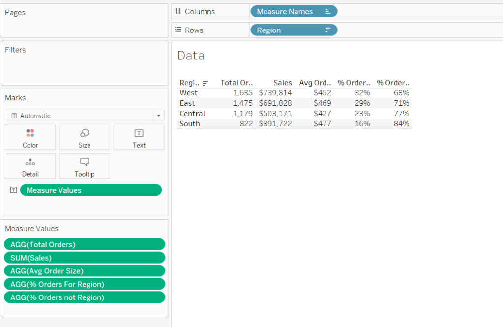
After connecting to the data, make sure all the fields are defined as dimensions (above the Measure Names line on the data pane) – if they aren’t drag them up. The only field in the Measure Values section should be the count of the records.

We first need to identify how many times each part was recorded in a strike (or not). Drag Part to Rows and Struck? to Columns. Create a new field

# Strikes

COUNTD([Strike ID])

Add to Text. This gives our basis for the inner ring.

The True values above, form the basis for which we then want to understand the split between whether the struck part was then damaged or not. On a new sheet, add Part to Rows and Damaged? to Columns, then create field

# Struck

COUNTD([Strike ID – Is Struck])

and add to Text. Additionally add row grand totals (Analysis menu > Totals > Show Row grand totals). The total for each row should match the True value from the previous sheet (pop the sheets side by side on a dashboard to sense check).

Once again, the Damaged? = True values, form the basis for which we then want to understand the split between whether the struck part was then substantially damaged or not. On a new sheet, add Part to Rows and Substantially Damaged and Part Damaged? to Columns, then create field

# Damaged

COUNTD([Strike ID – Is Damaged])

and add to Text and show row grand totals. Add this sheet to the dashboard too. The total for this sheet should match the True values from the Damaged sheet.

Building the Donuts

Now we’re happy with the numbers, we can start to build the viz. We’ll be using map layers for this, but as we don’t actually have a geometric datatype field in the data set, we need to create one. I’ll be following the core principles discussed in this blog post I wrote for the company I work for, Biztory. In the blog post, we’re just building 1 donut chart, so created a Zero point using MAKEPOINT(0,0). In this instance, I want multiple donuts arranged in rows and columns. This can be done in 2 ways:

  1. use the MAKEPOINT(0,0) method and then create 2 dimension fields added to Rows and Columns that represent the row and column for each Part (akin to what we do when building trellis/ small multiple charts) or
  2. use the MAKEPOINT method to define the point to position the donut. This is the method I’m using, but will break the fields required down, so it’s clear.

Create a new field

Row

CASE [Part]
WHEN ‘Engine’ THEN 1
WHEN ‘Nose’ THEN 1
WHEN ‘Windshield’ THEN 1
WHEN ‘Lights’ THEN 2
WHEN ‘LandingGear’ THEN 2
WHEN ‘Radome’ THEN 2
WHEN ‘WingOrRotor’ THEN 3
WHEN ‘Fuselage’ THEN 3
WHEN ‘Propellor’ THEN 3
WHEN ‘Tail’ THEN 4
WHEN ‘Other’ THEN 4
END

Column

CASE [Part]
WHEN ‘Engine’ THEN 1
WHEN ‘Nose’ THEN 2
WHEN ‘Windshield’ THEN 3
WHEN ‘Lights’ THEN 1
WHEN ‘LandingGear’ THEN 2
WHEN ‘Radome’ THEN 3
WHEN ‘WingOrRotor’ THEN 1
WHEN ‘Fuselage’ THEN 2
WHEN ‘Propellor’ THEN 3
WHEN ‘Tail’ THEN 1
WHEN ‘Other’ THEN 2
END

Ensure both of these are dimensions, by dragging above the Measure Names on the data pane if required. These fields are simply ‘hardcoding’ the position of each Part (and can be used if adopting the ‘trellis’ route).

Then create a field

Grid Position

MAKEPOINT([Column],[Row])

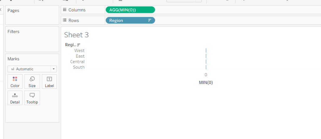
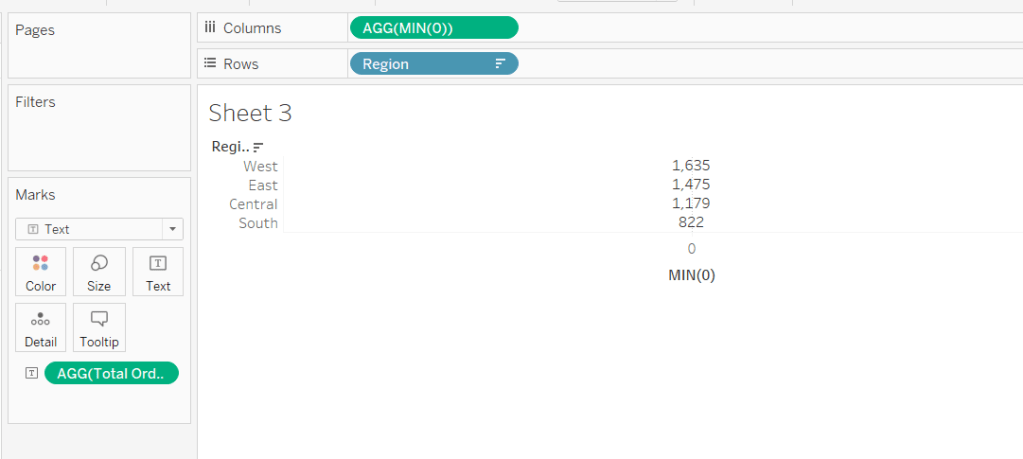
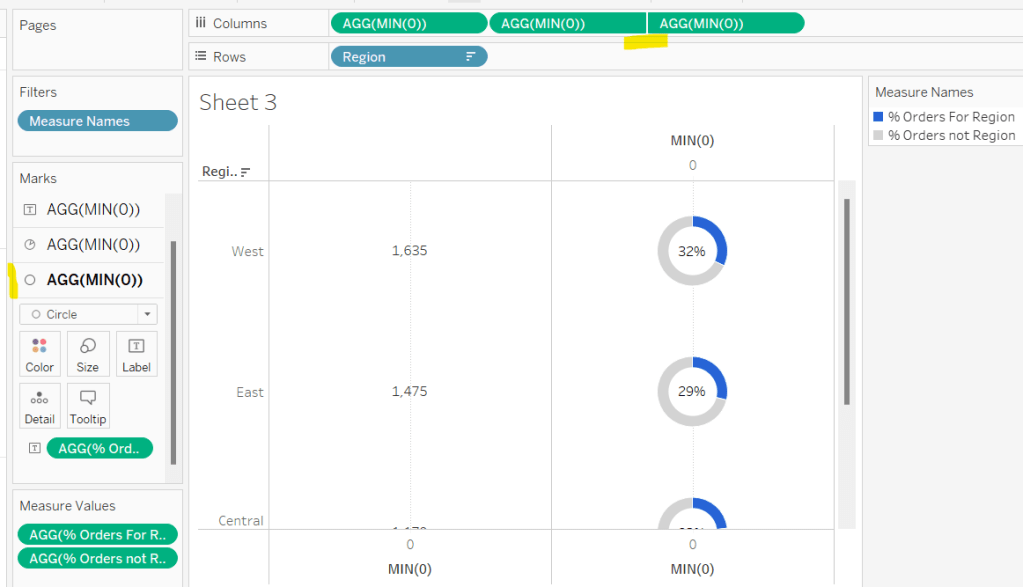
On a new sheet, add Grid Position to Detail and for now, add Part to the Label shelf so we can see what Part each mark represents.

Change the mark type to Circle.

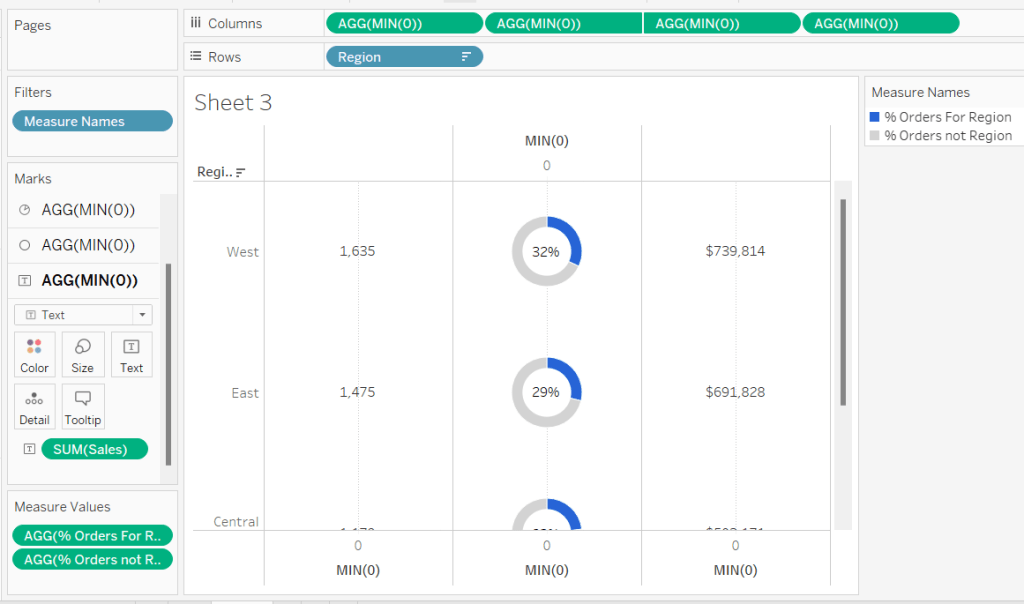
Drag another instance of Grid Position on to the canvas and drop when you see the option Add a Marks Layer. This will create another marks card called Grid Position (2).

Now we have 2 layers, we can reposition the marks. Note – doing the next steps before adding a 2nd marks layer, won’t let you then create any layers.

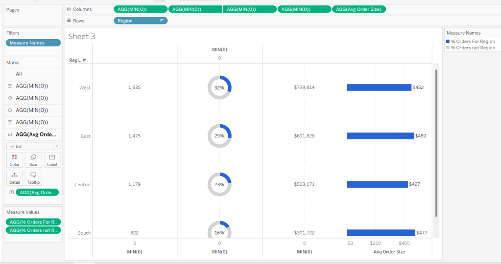
Use the swap axis button to change the axis so Latitude is on Columns and Longitude on Rows. Edit the Longitude axis (y-axis) and set the scale to be reversed. The Parts should all now be in the right place.

Now we can start to make the donuts. When using map layers, its good practice to rename the marks cards, so start by renaming the marks card Grid Position to be Centre and Grid Position (2) to be Struck Ring.

On the Centre marks card, change the colour to be dark grey (#44505b) and increase the size. Create a new field

Label – # Substantially Damaged

COUNTD(IF [Substantially Damaged and Part Damaged] THEN [Strike ID – Is Damaged] END)

Add this to the Label shelf and move Part to Detail instead. Position the label middle centre, but don’t adjust the font style in any way.

Create new fields

Tooltip – #Damaged

COUNTD(IF [Damaged?] THEN [Strike ID – Is Struck] END)

and

Tooltip – #Struck

COUNTD(IF [Struck?] THEN [Strike ID] END)

and add these to the tooltip shelf of the Centre marks card, and adjust Tooltip text – again don’t adjust the font style.

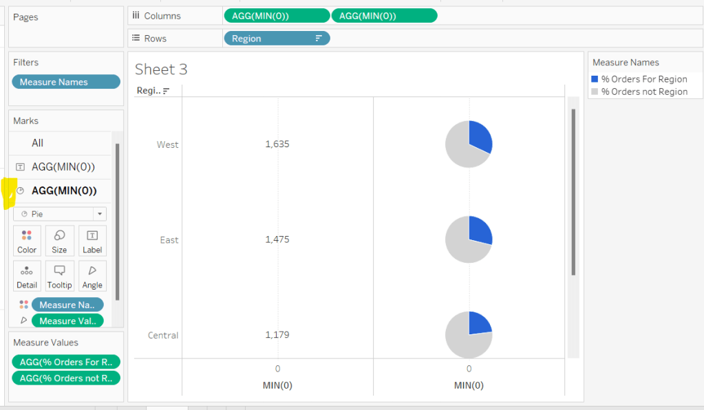
Click on the Struck Ring marks card. Drag it so it is under the Centre marks card. Add Part to Detail. Increase the Size until you can see a ring larger than the centre circle. Change the Mark Type to Pie and add #Strikes to the Angle shelf. Add Struck? to Colour. Adjust the colours, and re-order the colour legend so True is listed first.

Disable Selection on the Struck Ring marks card

Add another layer by dragging Grid Position on to the canvas. Rename this marks card to Inner Dark Grey Ring and move the card to the bottom. Add Part to Detail and then increase the Size. Change the mark type to Circle and set the colour to dark grey. Disable selection of the card.

Add another layer by dragging Grid Position on to the canvas. Rename this marks card to Damaged Ring and move the card to the bottom. Add Part to Detail and then increase the Size. Change the mark type to Pie, add #Struck to Angle and add Damaged? to Colour and adjust. Reorder the colour legend so True is listed first. Disable selection of the card.

Add another layer by dragging Grid Position on to the canvas. Rename this marks card to Outer Dark Grey Ring and move the card to the bottom. Add Part to Detail and then increase the Size. Change the mark type to Circle and set the colour to dark grey. Disable selection of the card.

Add the final layer by dragging Grid Position on to the canvas. Rename this marks card to Substantial Damage Ring and move the card to the bottom. Add Part to Detail and then increase the Size. Change the mark type to Pie, add #Damaged to Angle and add Substantially Damaged and Part Damaged? to Colour and adjust. Reorder the colour legend so True is listed first. Disable selection of the card.

Note – you may find you have to tweak the sizes of each layer – when published to Tableau Public, you can do this more accurately by setting a size % – on Desktop you just have to guess the slider position

Add in the custom theme

On the Format menu, select import custom theme and select the json file provided. When prompted select Override to apply the theme.

The font style and other properties of the chart should immediately update

Hide the axis, remove axis rulers and re-name the sheet.

Create the dashboard

Create a dashboard and set it to 1000 x 900. Add an Image object onto the dashboard, and select the background image provided, setting it to fit and centred. Remove the outer padding from both the image object, and the tiled container, so that the image object is exactly 1000 x 900.

You can see, that the labels for each donut, are actually part of the background image. So we now need to add the viz so it is positioned in the right place.

Change the dashboard objects to be ‘floating’ and add the Donut viz. Remove the Title, and delete the colour legends. Adjust the position and height/width to be x=448, y=104 and width=516 and height = 762 (this was done by trial and error – Iron Vizzers will have practiced so many times, they will know what they want these numbers).

But the background isn’t visible through the chart, so right click on the Donut sheet (while its on the dashboard), and Format and then set the background to be set to None.

And that is the crux of the challenge. I then added a floating title along with my standard footer. My published viz is here.

Happy vizzin’!

Donna

Can you filter a donut without highlighting the pie?

For this week’s challenge, Kyle looked to solve a problem that he’s seen discussed within another blog – how to solve a highlighting problem when filtering donut charts.

I’ve been away on a little holiday abroad for a family wedding, so am on catch up this week. So I’m going to make this as brief as I can as time is limited.

Building the donut charts

Use the steps described in this blog post I wrote for my company to build a donut chart using the dual axis method.

For the Category donut chart, you will need Category on Colour and Sales on Angle of the outer Pie Chart. For the inner circle, you will need to add Sales to Text. Adjust the text as required. Sales needs to be formatted to $ with 0 dp.

For the Sub-Category donut chart, you will need to add Category to Colour. Then add Sub-Category to Detail and click on the 3 dots to the left of the Sub-Category pill and change to also add to Colour.

To adjust the colours, edit the colour legend, select all the options within the same Category. Select a sequential colour palette that matches the core colour for the category, then select Assign Palette. The colours should change to a range of that colour.

Create a new field

# Products

COUNTD([Product ID])

and add this to the Angle shelf. Add Sales to the Tooltip shelf and adjust the tooltip.

For the inner circle, add #Products to Text. Adjust the text as required

Filtering the donut

Add the two sheets to a dashboard. Add a dashboard filter action

Filter Cat

On select of the Category donut, target the Sub-Category donut chart passing in all fields. Keep filtered values when selection cleared.

Stopping the Category donut from being highlighted

Create new fields

True

TRUE

False

FALSE

and add these to the Detail shelf on the All Marks card of the Category donut sheet.

Then create a dashboard filter action

Unhighlight

On select of the Category donut on the dashboard, target the Category donut sheet itself, passing in the fields Tue = False. Show all values when selection cleared.

Now when the Category donut is clicked on, the other segments won’t fade. However, the selection is still visible – the edges of the pie are displayed.

Stop showing the selected section of the pie

For this we employ a trick mentioned in the blog post referenced in the challenge. Create a new field

Dummy

‘Dummy’

and add this the Detail shelf of a new sheet. Change the mark type to polygon so nothing is visible.

Add this to the dashboard as a floating object – make it small and place somewhere inconspicuous

Whilst the selections will still be visible when testing on Desktop, once published to Tableau Public, the presence of the polygon forces the whole dashboard to be rendered server side rather than client side. This reduces the amount of interactivity, and consequently the pie chart segments don’t display when clicked.

My published viz is here.

Happy vizzin’!

Donna

Can you create donut charts exceeding 100%?

In 2024 the #WOW coaching crew has extended to include Yusuke Nakanishi (@YusukeNakanish3) and Yoshitaka Arakawa (@yoshi_dataviz) from the Japanese #datafam. This week Yusuke set this challenge asking us to build donut charts that represented when percentages were > 100%.

Building out the calculations

In the data set provided the Self-sufficiency ratio for food in calorie base [%] is a number that represents the actual % value ie 90 means 90%, 196 means 196%. To help me remember that, I formatted the field to be a number with 0 decimal places which had a % suffix.

But building the donut charts we need to ‘normalise’ the figures to represent a percentage out of 100. ie, if the value is 90%, we want 90%, but if the value is 196%, we want 96%. So I created

Self Sufficient %

([Self-sufficiency ratio for food in calorie base 【%】] %100) / 100

and then formatted this to a % with 0 dp.

but I can’t build a donut chart with just this value, I need to know the non self sufficient % too

Not Self Sufficient %

1-[Self Sufficient %]

and formatted this to be a % with 0 dp too.

Let’s put these into a tabular view. Add Prefecture to Rows and Measure Names to Columns. Add Measure Values to Text. Add Measure Names to Filter and restrict to the fields Self-sufficiency ratio for food in calorie base [%], Self Sufficient % and Not Self Sufficient %. Add Fiscal Year to Filters and restrict to FY2018. Sort the data by Self-sufficiency ratio for food in calorie base [%] descending.

You can see those rows where the Self-sufficiency ratio for food in calorie base [%], Self Sufficient % and Not Self Sufficient % is over 100% have a different value for the Self Sufficient %.

Showing the Fiscal Year as a filter the user can select, I can change to FY2019 and also see how these fields are behaving; ie when Self-sufficiency ratio for food in calorie base [%] is also over 200%, I’m getting the ‘remainder’ over 200 displayed ie 216% has a Self Sufficient % of 16%, which is what is needed for the ‘bonus’ challenge.

However, due to the way I’m building, I’m going to able to get the display working for the top & bottom 7 records regardless of year (making the build of the bonus challenge a bit easier).

So with this in mind, I now what to categorise the Self-sufficiency ratio for food in calorie base [%] based on what percentage range the values fall into.

% Bracket

FLOOR([Self-sufficiency ratio for food in calorie base 【%】] / 100)

This gives me values of 0, 1 and 2. By default this field will be created within the ‘measures’ section of the data pane (ie below the line). Drag it into the top section to convert it to a discrete dimension. Alias the values (right click -> Aliases) and set as below:

Then add to Rows.

and with the filter still set for FY2019, we can see the rows are categorised into 3 brackets.

Set the filter back to 2018. Now we want to restrict to the top and bottom 7 records only. For this I use Sets.

Create a set against Prefecture (right click the field > create > set).

Top 7

Top 7 records by Sum of Self-sufficiency ratio for food in calorie base [%]

Then create another set, this time for the bottom 7

Bottom 7

Bottom 7 records by Sum of Self-sufficiency ratio for food in calorie base [%]

Then create a Combined set (right click on one of the sets > create Combined set), that includes all values from both sets

Records to Include

Add this to the Filter shelf. By default it will show the records ‘in’ the set. However based on how the order of operations in Tableau works, this will apply the conditions based on the set first before it considers the year being filtered. Ie it will get the top and bottom 7 records based on the total sum of the Self-sufficiency ratio for food in calorie base [%] field for all the data in the data set, then filter to 2018. It means it could show some records that were in the top 7 overall, but not in the top 7 for 2018. To resolve this, and to ensure the data gets filtered by the Fiscal Year first, we need to add the Fiscal Year pill on the Filter shelf to context (right click pill and Add to Context). The pill will go grey.

Next we need a way to ‘categorise’ which rows are the top and which are the bottom. Add Top 7 to Rows which will split the rows into In or Out. Alias these values so In displays as Top 7 and Out displays as Bottom 7 (right click the text > Edit Alias).

Finally, when we build the viz, we need to ensure the 7 entries for each section align with each other. For this create

Top | Bottom Index

INDEX()

and convert the field to Discrete, then add to Rows before the Prefecture pill. Edit the table calculation so that it is computing based on the Prefecture and % Bracket pills only. This gives us an index from 1-7 for each set.

Building the Top & Bottom 7 Donut chart

On a new sheet, add Fiscal Year to Filter and set to 2018. Add the pill to context. Show the filter. Also add Records to Include to Filter.

Add Top 7 to Rows, then double click into rows and manually type MIN(0) to create a ‘fake axis’. Change the mark type to Pie.

Add Prefecture to Detail and Measure Values to Angle. Ensure only Self Sufficient % and Not Self Sufficient % are the only measures displayed (remove any others by dragging them out of the Measure Values box). Add Measure Names to Colour.

Add Top | Bottom Index to Columns and edit the table calculation so it is just computing by Prefecture. This should now give 7 columns of pie charts.

Add a Sort to the Prefecture pill on the Detail shelf, so it is sorting by the Self-sufficiency ratio for food in calorie base [%] field descending.

Add % Bracket to the Detail shelf, then click on the 3 dot icon to the left, and select the colour icon to add this pill to the Colour shelf as well as the Measure Names pill.

Re-edit the table calculation associated to the Top | Bottom Index pill so it is now also computing by the % Bracket field, so you get back to your correct top & bottom 7.

Adjust the order of the pills on the Colour shelf so that the % Bracket pill is listed before the Measure Names pill. Also adjust the order of the pills in the Measure Values box so Self Sufficient % is listed before Not Self Sufficient %.

Then adjust the colours on the colour legend as below and add a dark border to the marks (via the colour shelf).

Change the year filter to FY2019, and you can adjust the colours for the 200% entries too.

To make the ‘hole’ in the donut, double click into the Rows and add another instance of MIN(0). This will create a 2nd MIN(0) marks card.

On that marks card, move Prefecture from Detail to Label. Remove % Bracket, Measure Names and Measure Values. Add Self-sufficiency ratio for food in calorie base [%] to Label. Change the mark type to circle. Set the Colour of the circle to white. Align the label middle centre, and adjust the format/font to suit.

Set the chart to be dual axis and synchronise the axis. Adjust the Size of the pie chart mark independently from the size of the circle mark, so one is slightly larger than the other.

Finally tidy up the display by hiding the axis (uncheck show header), and the Top | Bottom Index field. Remove all gridlines, zero lines, axis lines/ticks and row/column dividers. Hide the In/Out Top 7 field label heading (right click label and hide field labels for rows. Update the title of the sheet so it references the Fiscal Year field. Change the filter back to 2018. Hide all tooltips.

Building the Legend

On a new sheet double click into Columns and type MIN(0.0). Add % Bracket to Rows. Change the mark type to square and add % Bracket to Colour and Label. Adjust colours to suit and add dark border to shape.

From the donut chart sheet, click on the Fiscal Year pill in the Filter shelf and set to apply to worksheets > selected worksheets and select the sheet you’re building the legend on. This will add the pill to this sheet too and changing the value on one sheet will impact the other.

Edit the axis so it is fixed to start at -0.1 and end at 1. This will shift the display to the left.

Hide the axis, and the % Bracket header column; remove all gridlines, zero lines, row/column dividers. Hide the tooltips.

Both the legend and the donut can now be added to a dashboard, and you’ve completed the main challenge. I chose to add the Fiscal Year filter to the display so the user could switch years if they wished.

The bonus challenge – Building the trellis chart

Because of how I’ve built the above, we’ve already done the hard work to handle the 200%+ data. The challenge here now is just to display all the 47 Prefectures for a given year in a 10 x 5 grid – a trellis.

So to build this, I started with the donut chart already built and duplicated the sheet.

When creating trellis charts, we need to create fields that represent which row and which column each Prefecture should sit in. There’s lots of blogs on creating trellis charts. As we know the number of rows and columns we need, I created

Cols

INT((INDEX()-1)%10)

Take the index of each Prefecture, decrement by 1 and find the remainder when divided by 10. This means the Prefecture with the highest % value at at position (rank) 1 will be positioned in column (1-0)%10 = 0. The Prefecture at position 11 will also be positioned in column (11-1)%10 = 0.

We also need

Rows

INT((INDEX()-1)/10)

Take the index of each Prefecture, decrement by 1 and divide by 10.

Convert both fields to be Discrete.

From the duplicated sheet, remove Top | Bottom Index from Columns and In/Out Top 7 from Rows. Remove Records to Include from Filter. Don’t panic if things look odd!

Add Cols to Columns. Adjust the table calculation to compute by both %Bracket and Prefecture. Specify the sort order to be a custom sort on the field Self-sufficiency ratio for food in calorie base [%] descending.

Now add Rows to Rows and apply the same settings on the table calculation. If all is well, you should have all 47 donuts displaying in the correct order.

Hide the Cols and Rows headings, and you can then add this to another dashboard.

My published viz is here: Top & Bottom 7 | Trellis

Happy vizzin’!

Donna

Can you visualise orders?

For Luke’s first challenge of 2023, he asked us to recreate this visualisation which showed multiple chart types (donut charts and bar charts) within a tabular layout, all built on a single sheet.

As with most challenges, I’m going to first work on building out the calculations needed to provide the data being presented.

Building the calculations

Firstly we need to identify the number of orders, based on unique Order IDs

Total Orders

COUNTD([Order ID])

and then to get the average order value we need

Avg Order Size

SUM([Sales]) / [Total Orders]

format this to $ with 0 dp.

In order to build the donut chart, we will need two measures for each region; one which shows the % number of orders for that region, and one which shows the % number of orders across the remaining regions.

% Orders for Region

[Total Orders]/SUM({FIXED:COUNTD([Order ID])})

Format this to % with 0 dp

and then

% Orders for not Region

1 – [% Orders For Region]

format this to % with 0 dp.

Pop all these out in a table along with Sales formatted to $ with 0 dp, and Sort the Region field based on Total Orders descending.

Building the table view

Add Region to Rows and sort by Total Orders descending.

All the columns are going to be managed by what I refer to as a ‘fake axis’. Double click into the Columns shelf and type in MIN(0). This will create an axis.

Change the mark type to Text and add Total Orders to the Text shelf. Remove all the text from the Tooltip dialog box.

This is our 1st ‘column’ in the table.

Create another column by adding another instance of MIN(0) to Columns.

Change the mark type of this 2nd MIN(0) marks card to Pie Chart and remove Total Orders from the text shelf.

Add Measure Names to the Filters shelf, and ensure only % Orders for Region and % Orders for not Region are selected.

Add Measure Values to the Angle shelf of the pie chart, and add Measure Names to Colour. Adjust the colours to suit and ensure a white border is added (via the Colour shelf options). Again remove all the text in the Tooltip dialog.

Now add another instance of MIN(0) to Columns.

Change the mark type of this marks card to Circle and set the colour to white. Add % Orders for Region to the Label and align centre.

Now make this Min(0) pill to be dual axis and synchronise the axis. Reduce the size of the circle mark type marks card, so some of the pie chart is visible. Remove Tooltip text again.

Add another instance of MIN(0) for our ‘3rd’ column. Set the mark type to Text and add Sales to the Text shelf, and remove the tooltip text.

For the final column, add Avg Order Size to Columns. Change the mark type to bar. Reduce the size and adjust the Colour to suit. Add Avg Order Size to the Label and remove all tooltip text.

Remove all gridlines zero lines and column dividers. Add row dividers at the highest level so you have a divider per row. Uncheck Show Header on the first MIN(0) pill to hide the axes, and right click the Region column label and Hide field labels for rows.

This gives you the viz you need to add to a dashboard. Use a horizontal container with a blank and 4 text boxes positioned above the viz to provide the label heading to the columns.

OR…

you can do what I did, and having not noticed the comment about the textboxes, used further instances of MIN(0) to make every ‘column’ a dual axis so I could use the axis label for the secondary axis displayed at the top to provide the required labels.

I set the mark type of these additional MIN(0) axis to polygon, and ensured no other pills existed on the marks shelf. The tick marks on all the top and bottom axes had to be set to none, and the title on all the bottom axis had to be deleted.

The benefit of using the text boxes option is that you aren’t left with a ‘blank’ space underneath the chart. However wide your axis is at the top to display the labels, will be repeated as ‘blank space’ underneath the chart too (vote up this idea to prevent this).

My published viz is here.

Happy vizzin’!

Donna

Can you use set actions to create a reference date range?

There’s a lot packed into the challenge this week, which was “set” by Lorna Brown and Erica Hughes to test our Set Action skills. How detailed this blog will go, I have yet to decide… I’ve got a couple of hours to get this nailed, so it could get quite brief as we get towards the end 🙂

I’ve got 6 sheets/charts making up this dashboard, so my intention is to summarise each one, and I’ll define the various calculations that are going to be needed as we go.

  • The overall summary table
  • The selected months summary table
  • The trend line
  • The donut chart
  • The top 3 states table
  • The map
  • Adding the interactivity

The overall summary table

This challenge is focused on understanding the Sales per month. Whilst its possible to use the built in aggregation features of a date field, I often prefer to create explicit date fields at the level I require, so it’s easier to reference. Therefore, the first field I created for this challenge was

Order Date To Plot

DATETRUNC(‘month’, [Order Date])

This essentially ‘groups’ every order placed in a month to be tagged with the 1st of the month. I custom formatted this field to MMM yyyy (ie Oct 21).

For the overall summary table, I need to capture the total sales of the whole data set, and I use a Fixed LoD calculation for this.

Total Sales

{FIXED: SUM([Sales])}

This field is formatted to $0.00M

NOTE – I actually named this field <space>Total Sales<space> as I want to display the name of the field (the measure name) in the summary table, but the ‘selected months’ summary table also has a Total Sales measure which is a different calculation (see later). Adding the <spaces> is a sneaky way to get two fields with what appears to be the same name. As this field when displayed will be centred, the <spaces> aren’t noticeable.

We also need to get the monthly average sales for the whole data set

Average Sales by Month

AVG({FIXED [Order Date To Plot]: SUM([Sales])})

Format this to to $0.0K

We can now build the summary table by adding Measure Names to the Filter shelf and selecting these 2 fields. The placing Measure Names on Rows and Measure Names and Measure Values on Text. Reorder the measures as required, hide Measure Names on Rows and format the Text as required.

Change the title of the sheet to Superstore Sales, ensure the tooltip doesn’t display and remove all gridlines / row banding etc.

The selected months summary table

The core requirement of this challenge is to make use of set actions, so we’re obviously going to need a set which will contain the dates (months) the user will select on the chart. This set will be based off of Order Date To Plot. Right click on the field > Create > Set. Name it Order Dates To Plot Set and by default, select all the months between Oct 20 to Jun 21 inclusive.

Later I’ll describe how the values of this set will get updated, but for now, we need to get some information relating to the sales in these selected months.

Firstly, we want the total sales for the months in this set.

Total Sales

IF [Order Date To Plot Set] THEN [Sales] END

The default format for this field is set to $ with 0 dp.

Note – this is the other ‘total sales’ field mentioned earlier. This field name has no leading/trailing spaces.

To get the average, I needed a field just to store each member of the set (ie each selected month)

Selected Dates

IF [Order Date To Plot Set] THEN [Order Date To Plot] END

and with this I can then work out

Average Sales

AVG({FIXED [Selected Dates]: SUM([Total Sales])})

The final measure required for this section is the change within the date range, which is basically comparing the value of sales at the first month in the selection with the sales in the final month selected. We need a few fields to get to this.

Firstly, we want to identify the first and last months

Min Selected Date

{FIXED:MIN(IF [Order Date To Plot Set] THEN [Order Date To Plot] END)}

If the date is in the set, then return the date and then take the minimum of all the dates, and store against all the rows in the data. Similarly we have

Max Selected Date

{FIXED:MAX(IF [Order Date To Plot Set] THEN [Order Date To Plot] END)}

Putting this info into a table, you can see how the calculations are working. The values for the Min & Max dates are the same across every row.

Next we need to get the Sales at the min & max points, and spread that value across all rows

Sales at Min Date

{FIXED: SUM(IF [Order Date To Plot]=[Min Selected Date] THEN [Sales] END)}

Sales at Max Date

{FIXED: SUM(IF [Order Date To Plot]=[Max Selected Date] THEN [Sales] END)}

Now we can work out the difference

Change within Date Range

([Sales at Max Date]-[Sales at Min Date])/[Sales at Min Date]

format this to a percentage set to 1 dp

Finally, we need to know the number of months in the set, which is displayed in the title of the monthly summary sheet.

Months in Set

{FIXED: COUNTD(IF [Order Date To Plot Set] THEN [Order Date To Plot] END)}

If the date is within the set, then capture the date, and the count the distinct set of dates captured.

Make this a discrete field (move from the measures section at the bottom of the data pane to the dimensions section at the top (above the line), and add to the tabular view

Now we can build the summary sheet.

Add Measure Names to the Filter shelf and this time filter by Total Sales, Average Sales and Change within Date Range. Add Measure Names to Rows and Measure Values to Text. Reorder the measures.

Format the Total Sales to be in $K, by selecting the Format option from the context menu of the Total Sales pill on the Measure Values shelf (hover on the pill and click the carrot/down arrow that appears – by formatting this way, we’re changing the display of this field for this sheet only).

Add Min Selected Date and Max Selected Date to the Detail shelf and set to be Exact Date. Format both these fields via the pill context menu to be the ‘March 2001’ format

Also add Months in Set to the Detail shelf.

Adjust the title of the sheet as below

Finally you need to set the background of the worksheet to the relevant purple (I used #8074a8), adjust the colours of all the fonts to white and adjust the size/style of the fonts in the table. Remove all gridlines/row banding etc, and you should have something like below

The Trend Line

By this point we’ve built all the calculated fields we need for this chart. This is a dual axis line chart, as we want the colour of the line for the selected dates to be different from the non selected ones, and we want to display a label for the highest sales in the selected timeframe.

  • Add Order Date to Plot to Columns, and set as a Continuous (green) pill set to Exact Date
  • Add Sales to Rows
  • Add Total Sales to Rows
  • Make the chart dual axis, and synchronise axis.
  • Adjust the colours of the Measure Names colour legend
  • On the Label shelf of the Total Sales marks card, set to label the maximum value only
  • On the All Marks Card, add Min Selected Date and Max Selected Date to the Detail shelf and set to Exact Date.
  • Right click on the Order Date To Plot axis and Add Reference Line
  • Create a reference band that starts at the constant Min Selected Date, ends at the constant Max Selected Date, is bounded by dotted lines and shaded between
  • Hide the Sales and Total Sales axis, format tooltips and adjust the row & column dividers.
  • Change the title and you should get to

The donut chart

Donut charts are 2 different sized pie charts on top of each other, created using a dual axis chart. On the Rows shelf type in MIN(0). Then type the same next to it. This gives you two axis and two marks cards.

We only care about information related to the selected dates for this chart, so we can add Order Date To Plot Set to the Filter shelf, which by default will just restrict the information to the data ‘in’ the set.

Change the mark type of the 1st MIN(0) marks card to Circle and add Sales to the Tooltip shelf. Adjust the size of the charts/mark.

Change the mark type of the 2nd MIN(0) marks card to Pie and add Sales to the Angle shelf. Add State to the Detail shelf. Sort the State field by Sales descending.

Note – the circles might look the same at this point, but if you hover over the bottom one, you should see that it’s segmented by State.

We need some new fields now to help us identify the top ranking states.

Sales Rank

RANK(SUM([Sales]))

This is a table calculation, so it’s best to see how this field will work in a table view – build one out as below, and set the table calculation on the Sales Rank field as shown

We’re now going to ‘group’ the ranks into the top 3 and everything else

Sales Rank Group

IF [Sales Rank]<=3 THEN [Sales Rank] ELSE 10 END

We can now use this Sales Rank Group field to colour the pie chart. On the 2nd MIN(0) marks card, add Sales Rank Group to the Colour shelf. Adjust the table calculation to compute using State as above, then change the field to be Discrete (blue). Adjust the colours to suit.

Now make the chart dual axis, and synchronise the axis. Adjust the size of the 1st MIN(0) circle to be smaller than the pie. If it’s not showing, right click on the right hand axis and move marks to back. Colour the circle white. Adjust tooltips to suit and hide axis, column/row dividers etc. Update the title. You should have

The top 3 states table

  • Add Order Date To Plot Set to Filter
  • Add State to Rows and Sales to Text and sort descending.
  • Add Sales Rank to Filter and set to At Most is 3. This will just show the top 3 states.
  • Add State to Text
  • Add a Percent of Total Quick Table Calculation to the existing Sales field that’s on the Text shelf (via the context menu of the pill)
  • Add another instance of Sales back onto the Text shelf
  • Adjust / format the font size and layout of the fields on the Text shelf
  • Add Sales Rank to the Size shelf and set to be discrete (blue) and set the mark type to be Text. Adjust the size of the marks – it’s likely it’ll need to be reversed and the range adjusted.
  • Hide the State field on Rows, adjust the font colours, remove row banding and row/column dividers. You should end up with…

The map

  • Add Order Date To Plot Set to the Filter shelf
  • Add State to Detail – this should create a map (edit locations to be US if need be – Map -> Edit Locations menu)
  • Add Sales to the Colour shelf
  • Edit the colour range to a suitable purple range ( I set the darkest colour of the range to #6c638f)
  • Adjust the map layers (Map -> Map Layers) so only the option highlighted below is selected.

Adding the interactivity

Add all the sheets to the dashboard, using vertical and horizontal containers to arrange the relevant layout. Then add a Set Action (Dashboard > Actions > Add Action > Change Set Values). The Set Action should be configured as below :

And fingers crossed, you should now be able to select marks on the trend line and see all the other charts, except the initial summary table, all update. My published viz is here.

Happy vizzin’! Stay Safe!

Donna

Visualise Our Survey Data

This week, Ann Jackson set a table calculations based challenge, using the responses from a recent survey on #WorkoutWednesday, as the most requested topic was for table calcs!

There’s a lot of visuals going on in this challenge, and I’m shortly off on my holibobs (so will be playing catch up in a couple of weeks), so I’m going to try to pare down this write up and attempt just to focus on key points for each chart.

Donut Chart

By default when you connect, Respondent is likely to be listed in the ‘Measures’ part of the data pane – towards the bottom. This needs to be dragged into the top half to turn it into a dimension. You can then create

# of Respondents

COUNTD([Respondent])

which is the key field measures are based on throughout this dashboard.

When building donuts, we need to get a handle on the % of total respondents for each track, along with the inverse – the % of total non-respondents for each track. To do this I created fields

Total # of Respondents

TOTAL(COUNTD([Respondent]))

and then

Track – % of Total

[# of Respondents]/([Total # of Respondents])

along with the ‘inverse’ of

Non Track – % of Total

1-[Track – % of Total]

To then build the donut, we ultimately need to create a dual axis chart, with Which track do you participate in? on Columns and a MIN(1) field on Rows. Manually reorder the entries so the tracks are listed in the relevant order.

On the first MIN(1) axis/marks card, build a pie chart. Add Measure Names to the filter shelf and filter to the Track & Non Track % of Total fields. Set Mark Type to Pie Chart and add Measure Values to the angle shelf. Add both Which track do you participate in? and Measure Names to the Colour shelf. Set a white border on the Colour shelf. Reorder the entries in the colour legend, and set the colours appropriately.

The create another MIN(1) field next to the existing one on the Rows shelf

Set this marks type to circle, and remove all the fields from the colour & detail shelves. Set the colour to white. Add Which track do you participate in? and Track – % of Total to the Label shelf and format. Reduce the Size. Make dual axis, and synchronise. Further adjust sizes to suit.

Participation Bar Chart

Plot How often do you participate? against # of Respondents, and then add a Quick Table Calculation to the measure using Percent of Total. Manually re-sort the order of the entries, show mark labels and Colour the bars light grey. Apply relevant formatting.

Diverging Bar Chart

In this bar chart, the percentage of ‘agree’ responses are plotted to the right on the +ve scale and the percentage of the ‘disagree’ responses are plotted to the left on the -ve scale. The percentage of the ‘inbetweeners’ (neither agree nor disagree) is halved, and displayed on both sides. To address this, I created the following:

# of Respondents – Diverging +ve

CASE ATTR([Answer])
WHEN ‘Agree’ THEN [# of Respondents]
WHEN ‘Strongly Agree’ THEN [# of Respondents]
WHEN ‘Neither Agree nor Disagree’ THEN [# of Respondents]/2
END / [Total # of Respondents]

This is the % of total respondents for the ‘agree’ responses and half of the ‘inbetweeners’.

Similarly I then have

# of Respondents – Diverging -ve

(CASE ATTR([Answer])
WHEN ‘Disagree’ THEN -1*[# of Respondents]
WHEN ‘Strongly Disagree’ THEN -1 *[# of Respondents]
WHEN ‘Neither Agree nor Disagree’ THEN ([# of Respondents]/2) * -1
END) / [Total # of Respondents]

which is doing similar for the ‘disagree’ responses, except all results are multiple by -1 to make it negative.

The Question field is added to the Filter shelf and the relevant 5 questions are selected. Answer is also on the Filter shelf with the N/A answer excluded.

Add Question to Rows (and manually sort the entries), then add # of Respondents – Diverging -ve and # of Respondents – Diverging +ve to Columns and add Answer to the Colour shelf. Manually resort the entries in the colour legend and adjust the colours accordingly.

Make the chart dual axis, and synchronise the axis. Change the mark type back to bar and remove Measure Names from the colour shelf if it was added. Edit the bottom axis to fix the range from -0.99 to 0.99 and amend the title. Format the axis to display as percentage to 0 dp. Hide the top axis.

Additionally format both the measures to be percentage 0dp, but for the # of Respondents – Diverging -ve custom format, so the negative value is displayed as positive on the tooltip.

Adjust formatting to set row banding, remove gridlines etc and set tooltips.

Vertical bar chart

The best way to start building this chart is to duplicate the diverging one. Then remove both measures from the Columns shelf and add Answer to Columns. Manually re-sort the answers. Add # of Respondents to Rows and add a Quick Table Calculation of percent of total.

Show the marks label, and align bottom centre, and match mark colour. Hide the axis from displaying, and also hide the Question field (uncheck show header). Update the Tooltip.

Heatmap

Right click on the Question field > Aliases and set the alias for the relevant questions

Also add Question to Filter and select relevant values. Add Answer to Filter too and exclude NULL.

Add Question to Columns and add Answer to the Text shelf. Add # of Respondents to the Text shelf, and set to Percent of Total quick table calculation. Edit the table calculation to compute using the Answer field only

We need to get each of these columns ‘sorted’ from high to low – we want to rank them. To do this, add # of Respondents to Rows, then change it to be a blue discrete pill. Add a Rank quick table calculation and once again set to compute by Answer only. Also set the rank to be Unique

Now change the mark type to square, and then add the # of Respondents percent of total field onto Colour as well as Text (the easiest way to do this to retain all the table calc settings, is to hold down Ctrl then click and drag the pill from the Text shelf onto Colour. This should duplicate the pill.

Format the % of total displayed to be 0dp, and adjust the label. Change the Colour to use the purple range and set a white border too. Hide the ‘rank’ field from displaying and hide field labels for columns too.

The dashboard

I used a vertical container then added the objects as required, using nested horizontal containers to organise the side by side charts.

To make the diverging bar and vertical bar charts look like they are one chart, adjust the padding of diverging bar chart object to have 0 to the right, and similarly, adjust the padding of the vertical bar to have 0 padding to the left.

I found it a bit fiddly to get the charts to line up exactly. Both charts were set to fit entire view. The diverging bar chart displays it’s title. I also displayed a title on the vertical bar chart, but made the text white so it’s invisible.

Dashboard filter actions are set against the donut and the participation bar charts.

The filter uses selected fields, which for the donut chart references the Which track do you partcipate in? field. A similar dashboard action needs creating for the participation chart as the source and references the How often do you partcipate? field.

A highlight dashboard action is required for the diverging and vertical bar charts. They only impact each other and should be set up as below on hover.

Hopefully I’ve covered everything… my published version is here.

Happy vizzin’! Stay Safe!

Donna

Can you hide a chart in map layers?

Candra set the challenge this week to use the new map layers to build a map display which, on click of a country, filtered the display to that country and additionally displayed a donut chart indicating the percentage of urban dwellers in that country.

If map layers are very new to you, then the webinar by Adam McCann referenced in the challenge, has some VERY useful pointers for this challenge (the workbook for that can be downloaded from here, as I found some things needed closer inspection).

I think this challenge is going to be best described by walking through the steps.

Building the 1st map layer

Double-Click on Country/Region to load a map, and change the mark type to (filled) Map. Add Region to the Colour shelf and assign the appropriate colours. Adjust the map background via the Map -> Map Layers menu and set the Style to dark, and remove all the selections against the Map Layers list

The intention is when a country is selected the map will ‘drill into’ /filter that country, and display additional information. We will drive this by a parameter, which will get set via a parameter action, but for now we’ll manually set the value.

Create a new string parameter, that is default to nothing/empty string/ ”, and then show this on your sheet.

pSelectedCountry

We need the 1st layer of the map to display, when there is no value in the parameter. We need a calculated field to help drive this.

All Countries

IF [pSelectedCountry]=” THEN [Country/Region] END

By default this will create a field of type ‘string’ but we need it to be a geographic data type. so change this as below.

Add this field to the Detail shelf of the map, and remove the Country/Region field that was automatically added when we first built the map.

Enter the name of a country, eg China, into the parameter. The map should essentially go blank (black screen).

Building the 2nd map layer

We need the country to display, if it’s entered into the parameter. For this, we need another calculated field

Selected Country

IF [pSelectedCountry]=[Country/Region] THEN [Country/Region] END

Once again change this to a geographic role data type of type County/Region.

Next click and drag this field onto the map, and drop it onto the Add Marks Layer option that displays. This will create a new Selected Country marks card, although nothing will obviously change on the map display itself.

Move the Selected Country pill to be on the Detail shelf instead, and add Region onto the Colour shelf. Change the mark type from circle to Map.

Now if you enter a county into the parameter, eg China, the display should ‘filter’ & ‘zoom in’ on China.

So what we have is the 1st layer only showing when no countries have been selected, and vice versa, the 2nd layer only showing when a country has been selected.

We need to now add further layers for the donut chart, which only want to show the country has been selected as well.

Building the 3rd map layer

A donut chart, in the past, is traditionally created by building a pie chart, then using a dual axis to add a circle, sized smaller that the pie chart, on top (see this Tableau KB for info). Rather than a dual axis, we’re going to use map layers – 1 layer for the pie chart, and then another layer for the central circle.

Keeping a country selected (so we can see what we’re building), drag Selected Country onto the map again to create another map layer. Change the mark type to Pie and increase the Size to as large as possible. Move Selected Country to Detail.

In the data set we have a field called Population Urban which stores the ‘percentage’ value of urban dwellers eg 0.17 is 17%. To create the angles for the pie chart, we need to know

Population Non-Urban

1-[Population Urban]

Drag Measure Values onto the Angle shelf. This will automatically add Measure Names to the Filter shelf. Edit the filter to just select the Population Urban and Population Non-Urban measures. Drag the Measure Names field that was also automatically added to the Detail shelf, to the Colour shelf. Adjust colours accordingly, and set the border of the pie chart to white (under the Colour shelf options).

Verify that if you set the parameter to empty again, the whole world map displays, and you can’t see any pie charts.

Building the 4th map layer

Now we need to make the donut hole. Once again, ensure a country is selected, so your pie chart is visible, then drag Selected Country onto the map again, and drop to add another map layer.

This time, move the Selected Country field onto the Detail shelf, add Region to the Colour shelf, and adjust the size of the circle, so its smaller than the pie. Set the border of the circle to be white again too,

Add Population Urban onto the Label shelf, and format to a percentage with 0 dp. The best way to do this, is to format the Population Urban measure in the data pane (right click->default properties -> number format).

At this point you’ll notice the number is huge… we need to add Year to the Filter shelf, and select 2012.

Align the label to be middle centre, and adjust the font to be much bigger text. Add ‘urban dwellers’ underneath.

Once again, verify you get the expected behaviour as you change the values in the parameter from nothing to Russia or China etc.

The final step on this sheet is to add text to the Tooltips. Unlike when working with dual axis, you don’t have an All marks card, so you’ll need to add the required fields (Country/Region, Region, Population Total (formatted to Millions with 0dp), Population Urban to the Tooltip shelf on each of the relevant layers.

Setting the parameter interactively

Create a dashboard sheet, and add the map sheet you’ve built. Then create a dashboard action which sets the pSelectedCountry parameter, impacting the All Countries field, and that when the selection is cleared, the value is reset to ”.

My published viz is available here. Enjoy!

Happy vizzin’! Stay Safe!

Donna

What is our daily fulfilment rate by region?

This week Luke challenged us to create Donut Charts in Tableau, but added additional requirements to make it just a bit spicier. The full details are here.

Taking inspiration from Ann’s challenge the week before, Luke provided an advanced version to incorporate grey circles for each date when there were no orders, but stated this should be achieved without any data duplication or densification. Deep down, I knew Luke really meant ‘only one sheet’, but he didn’t state this, so my initial interpretation was to tackle the challenge in a similar way to Ann’s, and use 2 sheets; a background with all the grey circles displayed, and a foreground with the donuts/green circles, and float one over the other. This week, while still tricky, I managed to get them aligned, so that was the version I published and released.

I documented this floating technique last week, here, so have no plans to repeat, except to state that I got all the dates to display by creating a Baseline Date field of

MAKEDATE(2019, MONTH([Order Date]), DAY([Order Date]))

which is basically setting all the dates in the dataset to the same year. I then used this date to build my background viz, and as there was an order in every region for the day/month combination, I didn’t get any gaps. If the dataset didn’t exhibit this behaviour, this technique would not work, so it isn’t the most robust solution.

Right, now I’ve finished talking about that, let’s get onto building the chart…

Fixing the report date

Luke stated the report should be based on the last 7 days from 6th Nov 2019, so this date had to essentially be ‘hardcoded’ into the report. The easiest way to do this in a way that could be quickly changed if need be, was to create a parameter, Report Date, defaulted to 6th Nov 2019.

Restricting to 7 days

I created a calculated field to limit the data just to the days I was interested in

Dates to Include

[Order Date] >= DATEADD(‘day’, -7, [Report Date]) AND [Order Date]<= [Report Date]

Determining the % of orders shipped

This required a few calculated fields. First up, we needed to know if the order had shipped before the report date or not

Has Shipped?

[Ship Date]<= [Report Date]

# Shipped

IIF([Has Shipped?],1,0)

This returns 1 or 0 depending on whether the order has shipped before the report date or not. This field when added to the viz, can then be aggregated (summed) to provide a count of the orders that have shipped.

% Shipped

SUM([# Shipped])/SUM([Number of Records])

How many shipped as a proportion of all records. NOTE – in this solution, an order equates to a row in the data set. However technically, an order can contain multiple rows, so when counting orders, you could think you need to COUNTD([OrderID]). This is certainly valid, and IMO more accurate, but things do get a bit more complex this way. Luke had counted rows, so I decided to work with getting the data to match his solution.

Finally we needed to know if the orders had been fully shipped or not, as this is what will determine whether we’re showing a green circle with a tick, or a donut.

Fully Shipped?

[% Shipped]=1

Building the Donuts

I’ve worked with donut charts before, so knew that the trick was in using a dual axis technique to show a pie chart with a smaller circle mark on top.

I also needed ‘axis’ to work with, so incorporated our old friend MIN(0), and added 2 instances as synchronised dual axis like below:

The first instance, I changed to be of mark type Pie chart, adding SUM([Number of Records]) to the Angle shelf, and Has Shipped? to the Colour shelf. The colours were set to green if Has Shipped? was true and grey otherwise. The colours were reordered, so True is listed first, so the green starts at 12 o’clock.

On the second instance, I changed the mark to be a circle, adjusted the size so it was smaller, and added Fully Shipped? to the Colour shelf. This time the colour is set to green if true, but white if false.

For the labels, I created 2 calculated fields :

Label Tick

IF [Fully Shipped?] THEN ‘✓’ END

Label % Shipped

IF NOT([Fully Shipped?]) THEN [% Shipped] END

and added these side by side to the Label shelf of the Circle mark. The font was adjusted to fit, and centre aligned.

Removing the column/row labels, hiding some of the pills and formatting the axis/gridlines etc, and the core of the viz is built. This would achieve the ‘standard’ solution.

Date Format

The order date was set to a custom format of mmm d, ‘yy to get the desired display.

Displaying the grey circles

As stated above, I originally used the 2 sheets & floating technique to show the circles within the gaps.

After publishing, I had a look at Luke’s solution to see how he’d tackled it.

However much I stared at his workbook though, I could not see what he’d done. All I could tell by playing around was that there were no further marks than what I had already got displayed.

Then Rosario Guana posted up her solution, so I checked hers out too…. still couldn’t see it. I went through every menu option I could think of, trying to find what the secret was…..

Eventually I pinged Rosario a message… background image was the response.

Doh! I don’t use these often, well actually I’ve only used it once on another #WorkoutWednesday challenge that Rody Zakovich set sometime ago. Tableau’s help on using Background Images (which you often associate with maps, and hence is under the Maps menu option), is here.

So now I had the clue, what did I need to do….

First up, I needed an image to use. As I’d already downloaded Rosario’s workbook, I used the one in her workbook.

Secondly, I needed ‘proper’ pills to map the co-ordinates of my image to, my ‘typed in’ MIN(0) wouldn’t suffice. So I created

Col

0.0

Row

0.0

I then rebuilt the viz with Col (set to be a dimension), and added Row to the rows shelf (again set to be a dimension). I hid all the headers again

I then added the image via Map > Background Image > <Data source name>, then Add Image, and applied settings below

The sizes just then needed to be adjusted to fit, but this is best done when displayed on the dashboard itself, as what you see in the sheet view might not present the same when on the dashboard.

Both my versions of this challenge can be viewed here.

Happy vizzin’

Donna