Can you use containers and dynamic zone visibility?

This week’s #WOW2025 challenge was set live as part of TC25. Unfortunately, this year I couldn’t be there in person to meet everyone, which for the last 3 years has been my conference highlight 😦

Anyway, Kyle set the challenge, and conscious of time, provided a starting workbook, so the focus could be on the container and DZV functionality. For those who nailed this, he added some additional interactivity with dashboard actions.

So the first thing is to download the starter workbook from the challenge page.

I’m going to attempt to build this in the order of Kyle’s requirements.

Layout out the dashboard

So the requirement states that no floating objects are allowed. Typically when I build a dashboard for business purposes or where the layout is a little complicated, I always start by adding a floating container sized to the exact dashboard size and positioned 0,0. I then add tiled objects into it. Doing this means I don’t end up with Tiled container objects on my dashboard (or if any get added when legends/filters get automatically added, I just move any items I want to retain and then delete the Tiled container).

However, as Kyle says ‘no floating’, I will build adding to the ‘default’ dashboard which means there will be containers on there I don’t really want.

Now blogging about containers is usually very tricky as it’s hard to explain where things need to go. So I’ll be supplementing this with a lot of screen shots – fingers crossed following along works out ok!

To start, create a dashboard sheet and resize to 1200 x 900 as required. Observe the item hierarchy section of the Layout pane as this is where you’ll see all the containers and objects as we add them to the dashboard.
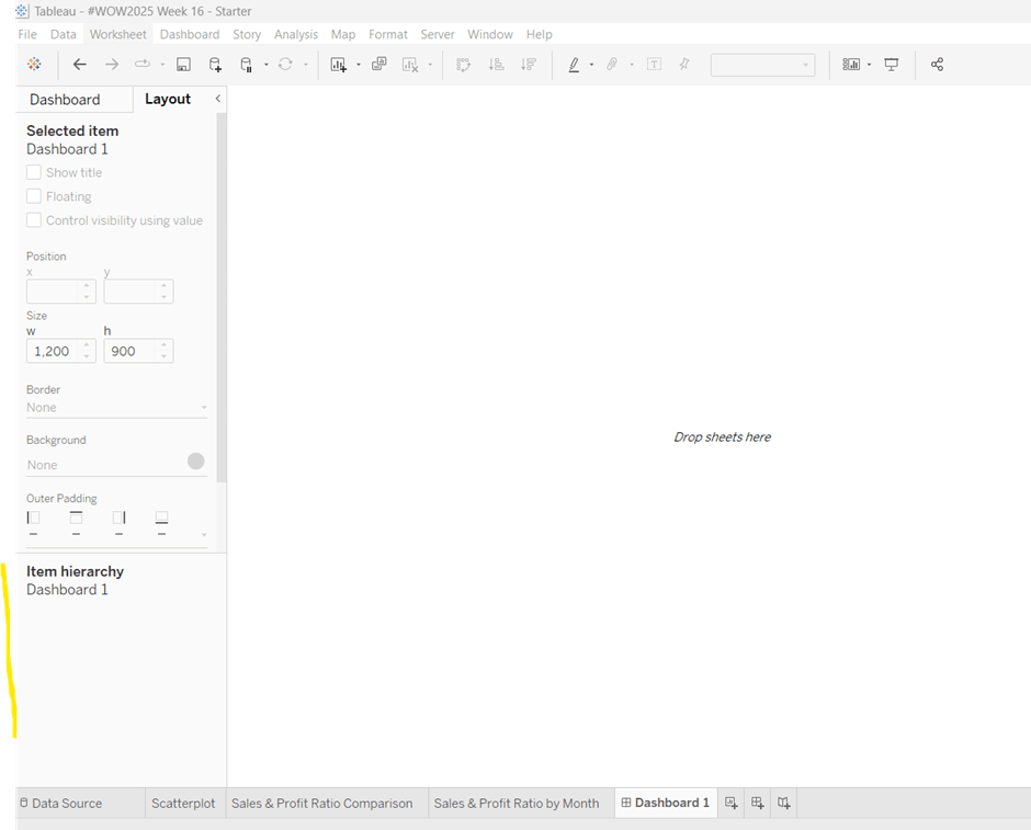
The main structure of the display is split into 2 columns, so start by adding a horizontal layout container to the dashboard. Once added, add 2 blank objects side by side to give the basic layout. Adding blank objects helps when positioning the required objects and is recommended when dealing with layout containers, especially if you’re new to them. They will ultimately be deleted as we go. Rename the horizontal container H – 2 cols or similar (right click on the container in the item hierarchy  > rename).
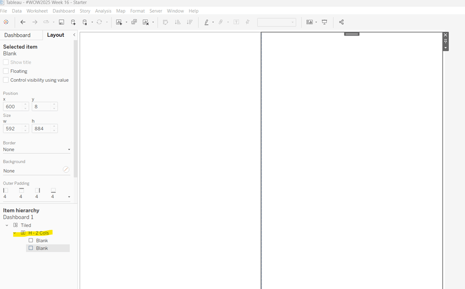
Notice how a Tiled container has now also appeared on the dashboard, even though we only added a horizontal container.

The first column of the dashboard contains 2 charts – the Scatterplot and the Sales & Profit Ratio Comparison sheets – stacked on top of each other. For this, add a vertical layout container between the two blank objects. Rename this V – Col 1.
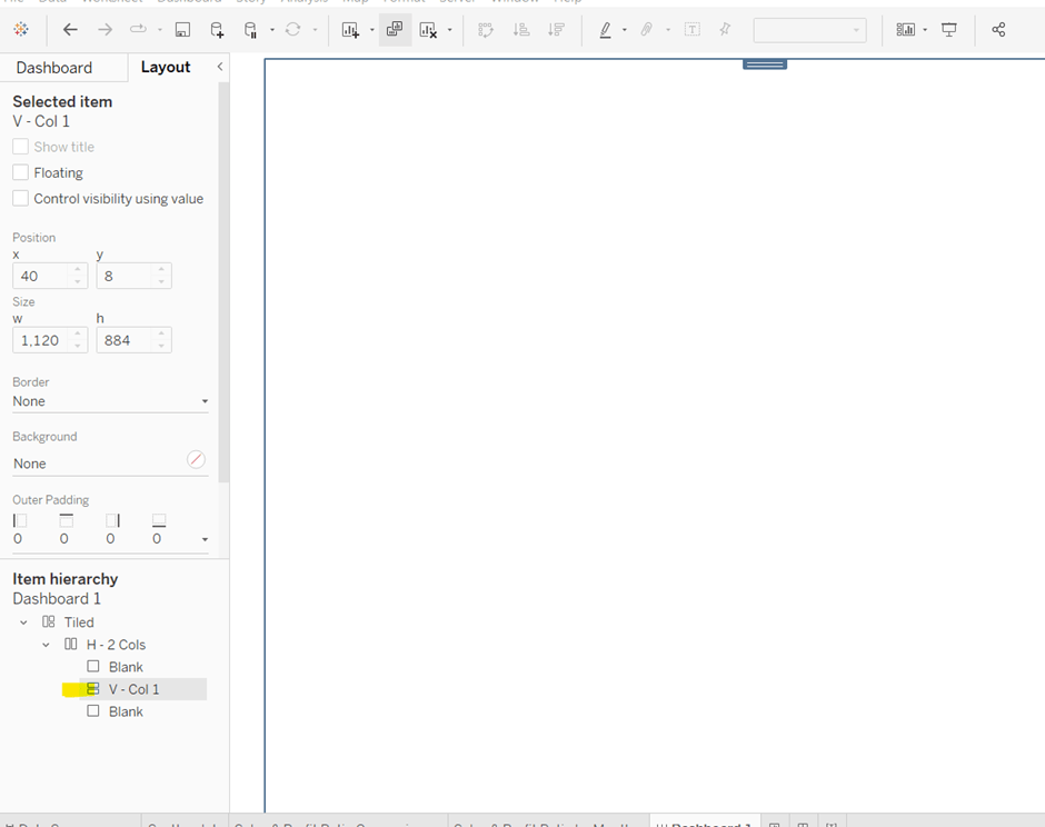
Add the Scatterplot sheet into the vertical container and then add Sales & Profit Comparison underneath it.
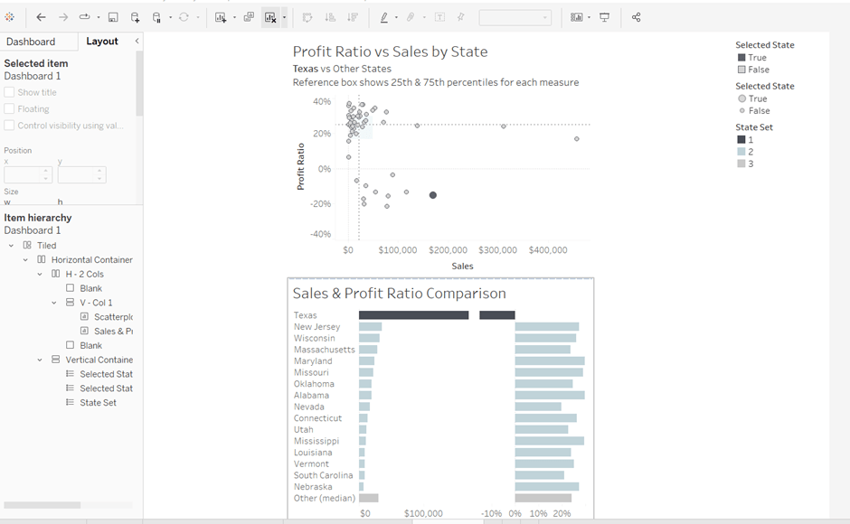
The various legends associated with these 2 sheets, automatically get added into their own vertical container on the right hand side. These aren’t required, so from the item hierarchy, select the Vertical container and then Remove from dashboard.
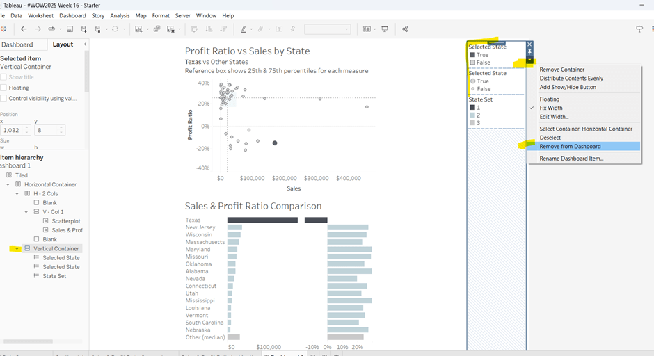
The right hand column of the display will show the Sales & Profit Ratio by Month sheet and another (hidden) chart that needs to be built.

Add another vertical container between the V – Col 1 container and the right hand blank object. Name this V – Col 2, and add the Sales & Profit Ratio by Month sheet and then another blank object underneath it. Once again remove the right hand vertical container that is automatically added with all the legends/filters.
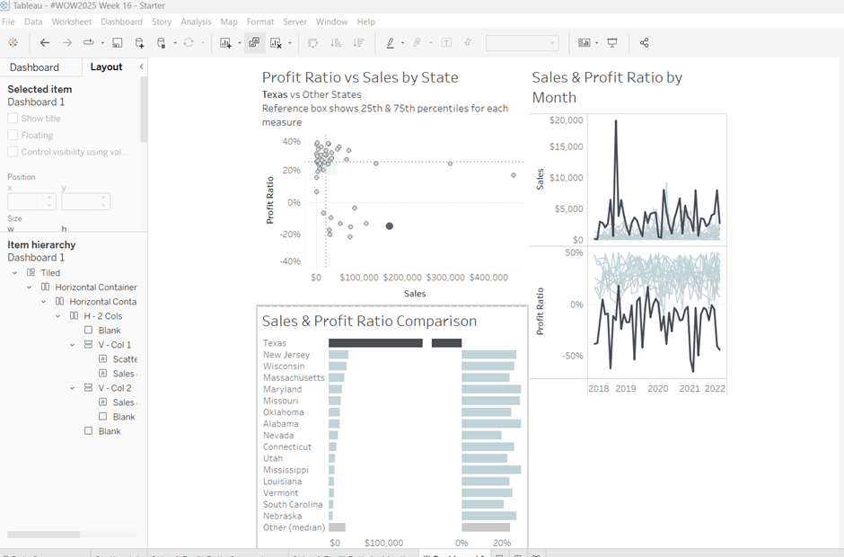
Now we have the ‘core’ layout, the 2 blank objects we added to the horizontal container, H – 2 Cols, right at the start, can be removed, so hopefully you should have a layout organised as below.
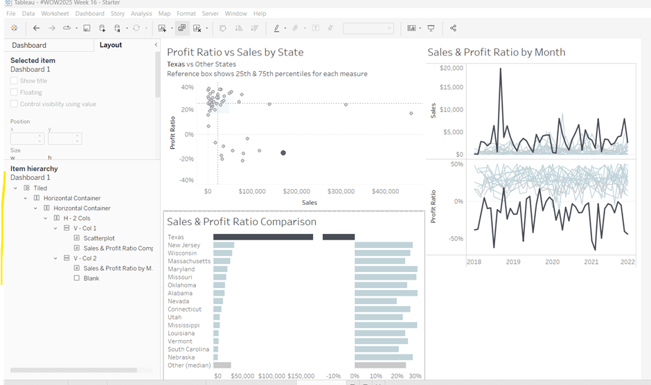
Now add the dashboard title (Dashboard menu > Show Title, and then update the text). This will automatically add a vertical layout container around all the existing contents.
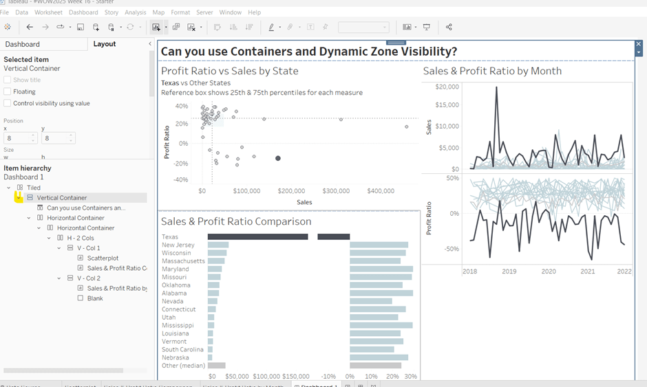
Building the Sales & Profit Ratio by Sub-Category bar chart

On a new sheet, add Sub-Category to Rows and Sales to Columns. Add Profit Ratio to Colour and adjust the colour legend to use the Red-Black Diverging colour palette. Hide the Sub-Category row label heading (right click > hide field labels for rows).
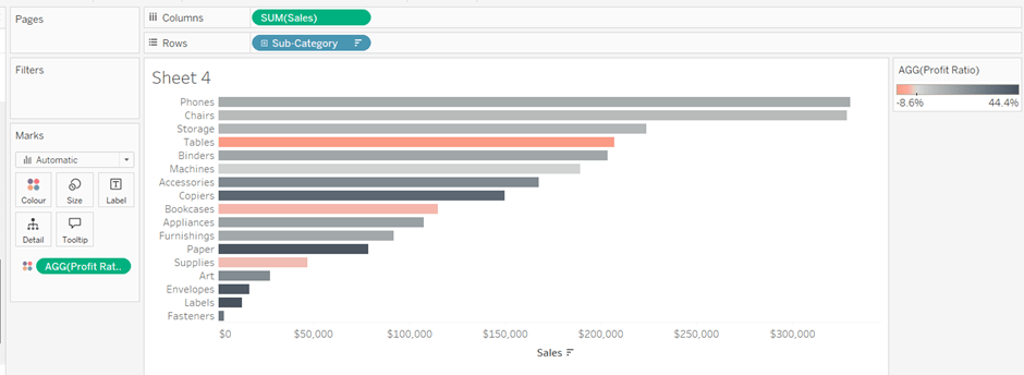
The bar chart needs to be filtered when a State in the Sales & Profit Ratio Comparison chart is clicked on, or when a Date is selected in the Sales & Profit Ratio by Month chart. However, I noticed when clicking around, that when clicking the Sales & Profit Ratio by Month chart, it filtered the above bar chart by both the State and Date. So based on this, create 3 parameters.

S&PR Comp State

String parameter defaulted to empty string
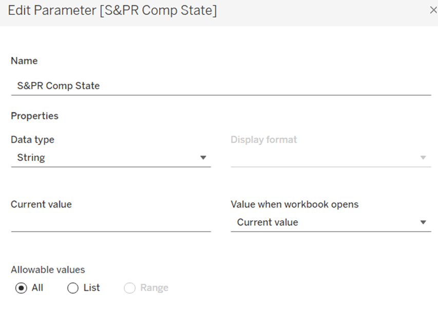
S&PR by Month State

String parameter defaulted to empty string

S&PR by Month Date

Date parameter defaulted to 01 Jan 1900 (essentially a null date)
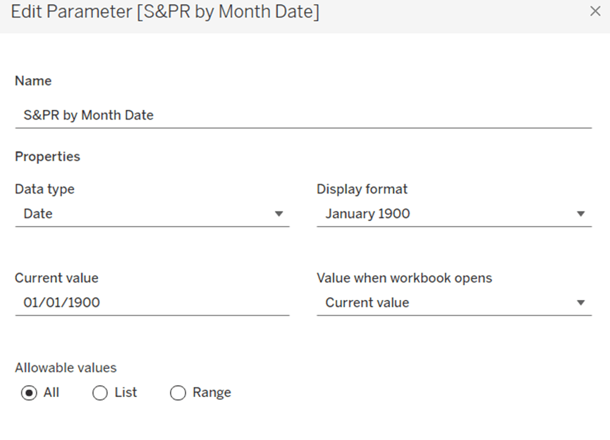
Show these parameters on the sheet.

We want to filter the chart if the S&PR Comp State has a value and the S&PR by Month Date is the ‘null’ date (which means we’ve interacted with the Sales & Profit Ratio Comparison chart), or if the S&PR Monthly State has a value AND the S&PR by Month Date has a value (which means we’ve interacted with the Sales & Profit Ratio by Month chart). So create

Filter – S&PR by SubCat

([State Name] = [S&PR Comp State] AND ([S&PR by Month Date]=#1900-01-01#))

OR

(([State Name] = [S&PR by Month State]) AND (DATETRUNC(‘month’, [Order Date]) = DATETRUNC(‘month’, [S&PR by Month Date])))

Enter a State name into the S&PR Comp State parameter (eg New Jersey), then add the Filter – S&PR by SubCat field to the Filter shelf and set to True. The chart should change.
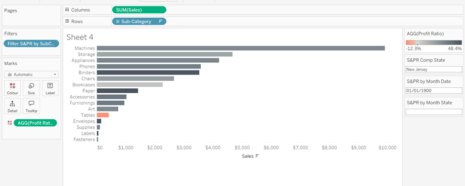
Verify the functionality by adding a state and date into the other parameters eg 01 March 2021 and Texas
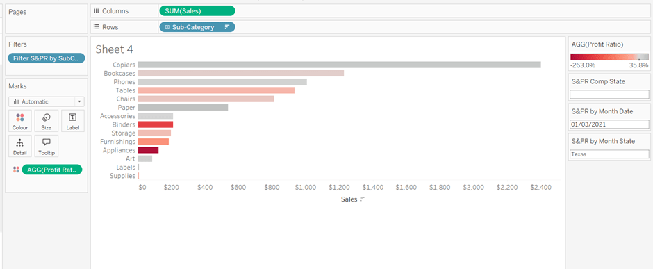
Empty the state parameters and set the date back to 01 Jan 1900. Name the sheet Sales & Profit Ratio by SubCat. The chart contents will disappear.

Creating a dynamic title sheet

Originally I hoped to do this without using another sheet and just using the title of the bar chart, but I need the date to show nothing rather than Jan 1900 depending on the user interactivity, so a new sheet is required.

But for it, we need some additional calculated fields.

State for Title

IIF([S&PR by Month State]<>”,[S&PR by Month State], [S&PR Comp State])

We only want to show the name of the state once, and both parameters may have it set.

Date for Title

IF [S&PR by Month Date]=#1900-01-01# THEN ” ELSE DATENAME(‘month’,[S&PR by Month Date]) + ‘ ‘ + STR(YEAR([S&PR by Month Date])) END

Line

IF [S&PR by Month Date]<>#1900-01-01# THEN ‘|’ ELSE ” END

Add all 3 fields to the Detail shelf of a new sheet. Change the mark type to polygon. Update the sheet title as below
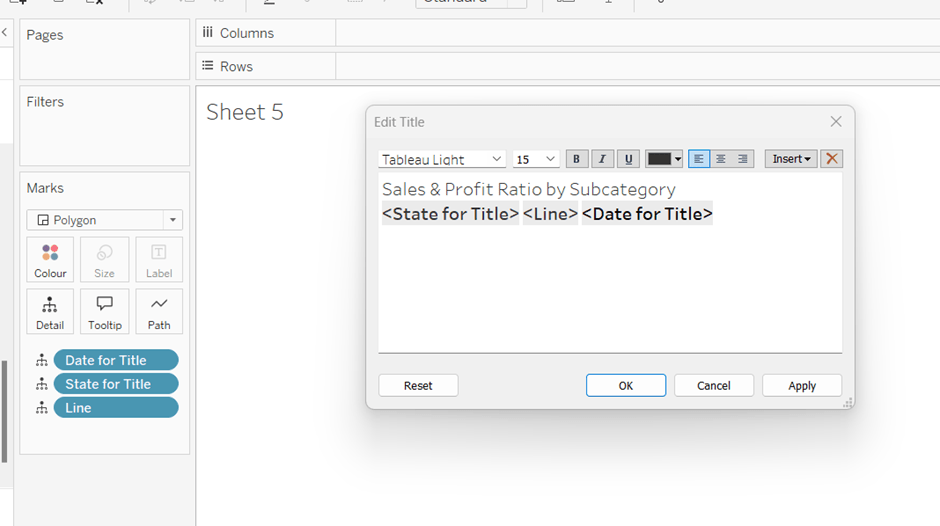
Name the sheet S&PR Title Sheet or similar

Adding the bar chart, title & legend to the dashboard

All 3 of these objects – the bar chart, the title sheet and the profit ratio legend need to show or hide based on interactivity. To do this in one step, we can encapsulate the 3 objects within containers within another ‘parent’ container and control the visibility on the ‘parent’ container.

Add a vertical container between the Sales & Profit Ratio by Month chart and the blank object. Name this V – S&PR SubCat Chart
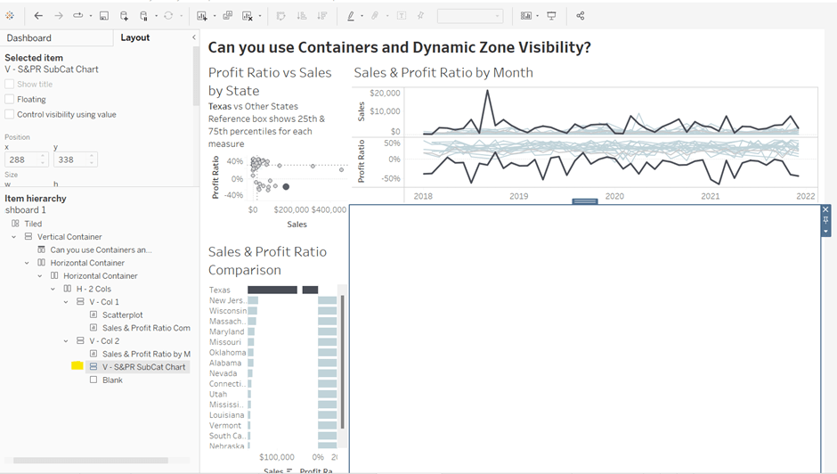
Add the Sales & Profit Ratio by SubCat sheet into this. Then add another horizontal container and place it above the Sales & Profit Ratio by Sub Cat chart (making sure it’s within the V – S&PR Sub Cat Chart container. Rename this H – S&PR Sub Cat Title.
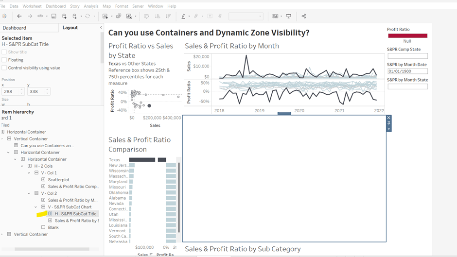
Add the S&PR by Title sheet into this horizontal container, and then click on the Profit Ratio legend on the right hand side and move this object to sit to the right of the title sheet. Then click on the right hand column containing all the remaining legends, and delete this container from the dashboard. Then remove the blank object that’s sitting beneath the Sales & Profit Ratio by SubCat sheet. You should have something like below…
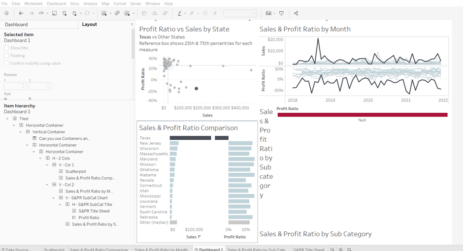
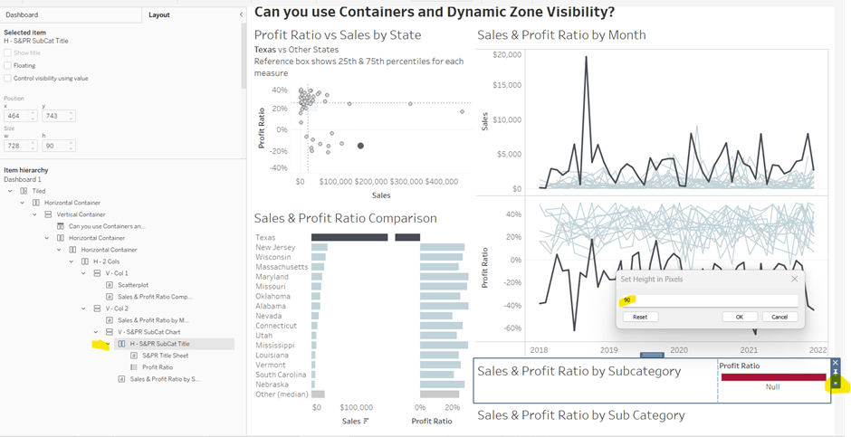
Adjust the width of the S&PR Title sheet so its wider. Set the sheet to Fit Entire View. Then select the H – S&PR SubCat Title container and edit the height to be 90 px.
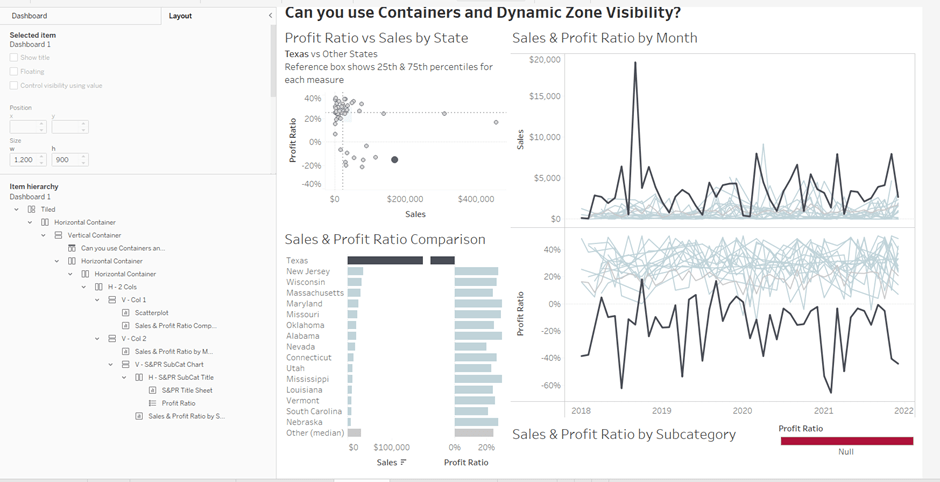
Hide the title of the Sales & Profit Ratio by SubCat sheet.
Hiding and showing the Sales & Proft Ratio by Sub Category section

Create a new calculated field

Show S&PR by Sub Cat

[S&PR by Month State]<>” OR [S&PR Comp State]<>”

On the dashboard, select the V – S&PR SubCat Chart container and on the Layout pane, check the Control visibility using value checkbox, and select the Show S&PR by Sub Cat field. Assuming all the parameters are set to their default values, then the whole section should disappear, although the container will still be selected.
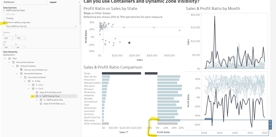
To make the section show, we need to set the parameters using dashboard parameter actions.

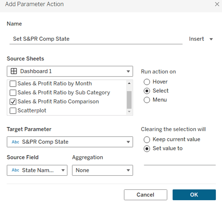
Set S&PR Comp State

On select of the Sales & Profit Ratio Comparison sheet, set the S&PR Comp State parameter passing in the value of the State Name field. When the selection is cleared, set the value back to <emptysrting>
Click on a row in the Sales & Profit Ratio Comparison bar chart, and the Sales & Profit Ratio by SubCat chart should display, filtered to that State, with the selected state name in the title.
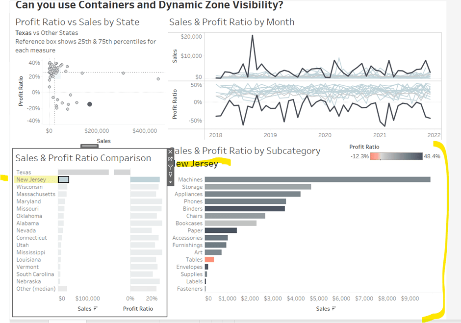
Click the state again, and the chart disappears.

Create 2 further dashboard parameter actions

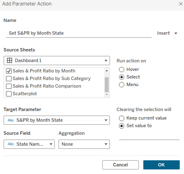
Set S&PR by Month State

On select of the Sales & Profit Ratio by Month sheet, set the S&PR by Month State parameter, passing in the value from the State Name field. When the selection is cleared, set it back to <emptystring>
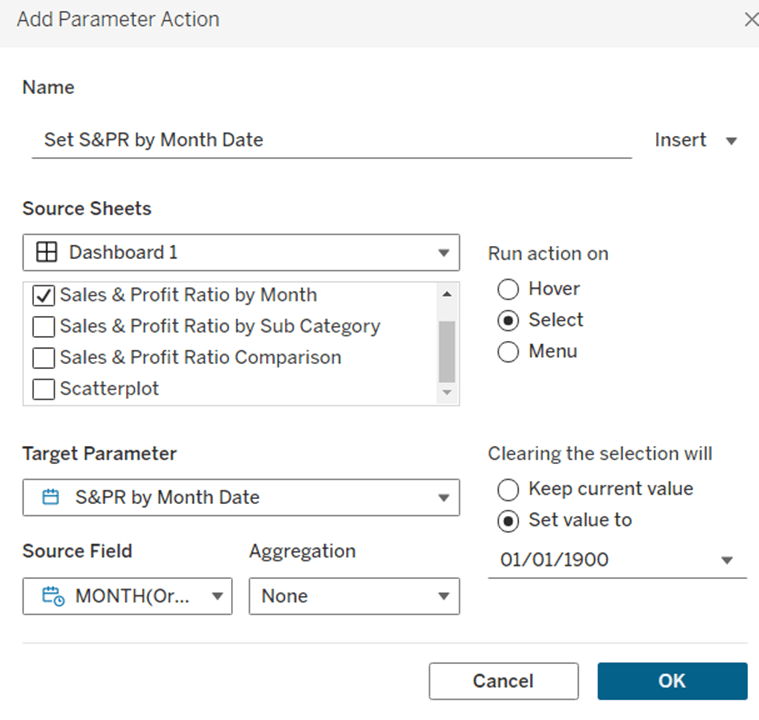
Set S&PR by Month Date

On select of the Sales & Profit Ratio by Month sheet, set the S&PR by Month Date parameter, passing in the value from the Month([Order Date]) field. When the selection is cleared, set it back to 01/01/1900
Now click on a point in the line chart, and the Sales & Profit Ratio by SubCat chart should display filtered to the relevant state and month
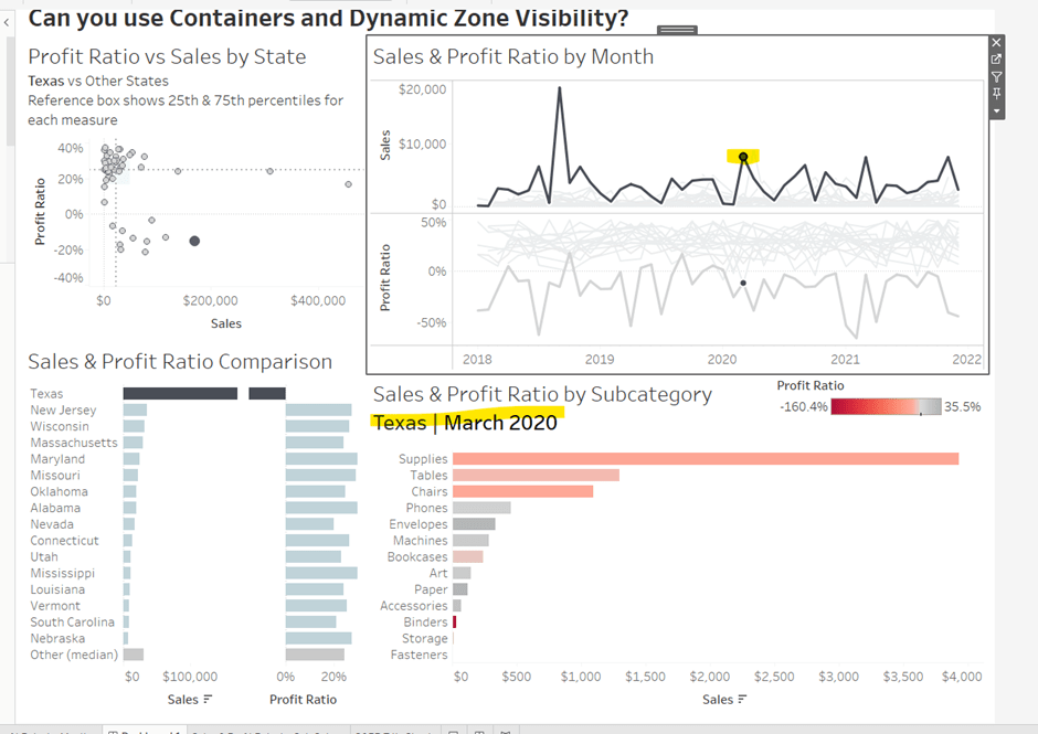
Adding the Additional Interactivity

When the Scatterplot is clicked, the State in the existing Scatterplot State parameter should be updated. Create a dashboard parameter action

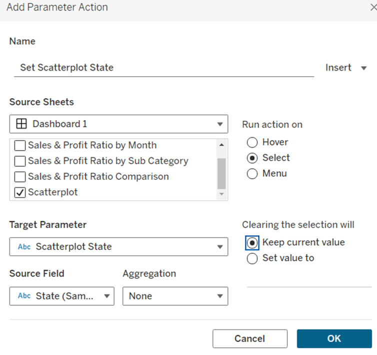
Set Scatterplot State

On select of the Scatterplot sheet, set the Scatterplot State parameter, passing in the value from the State field. When the selection is cleared, retain the value
If you click around the scatterplot, the Sales & Profit Ratio by Month line chart and Sales & Profit Ratio Comparison charts should update.

But we don’t want the other marks on the scatter plot to ‘fade’. To solve this, create a dashboard filter action.

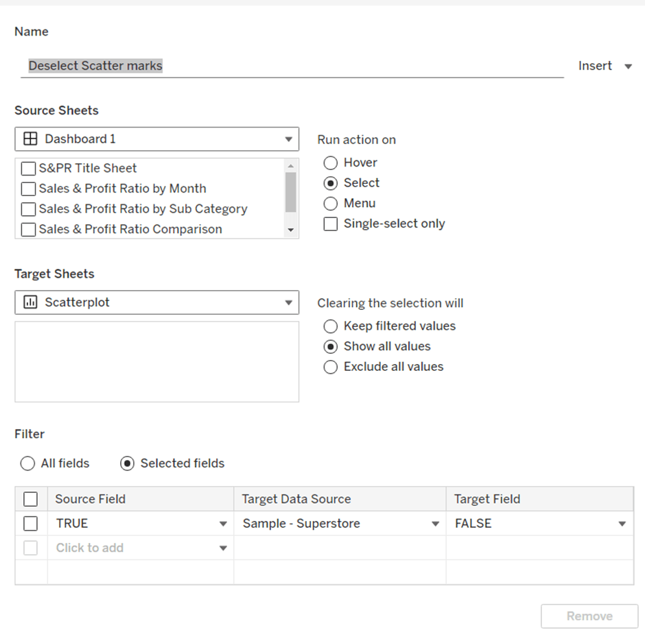
Deselect Scatter marks

On select of the Scatterplot sheet on the dashboard, target the Scatterplot sheet directly, setting the fields TRUE = FALSE. On clearing the selection, show all values.
Finally, the last requirement is to highlight the line in the Sales & Profit Ratio by Month chart associated to the State selected in the Sales & Profit Ratio Comparison chart. For this first create a dashboard set action to capture the selected state

Add State to Set

On select of the Sales & Profit Ratio Comparison sheet, target the State Name Set. Check the single-select only checkbox. Running the action should Assign value to set and clearing the selection should remove all values from set

Then add a dashboard highlight action

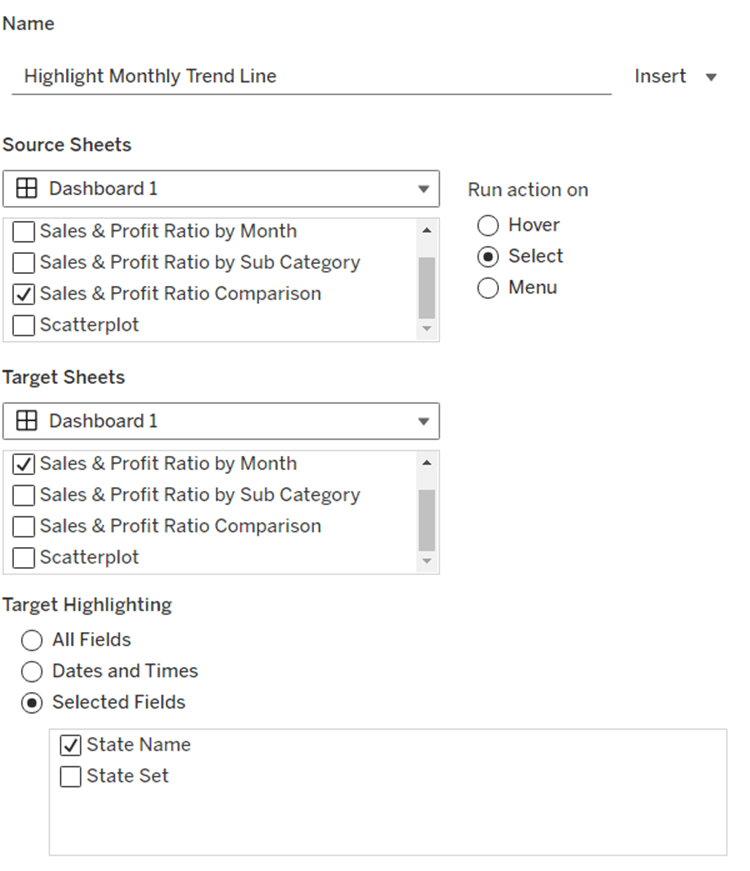
Highlight Monthly Trend Chart

On select of the Sales & Profit Ration Comparison sheet, target the Sales & Profit Ratio by Month sheet targeting the State Name field only
And hopefully, with all this, you should have a fully interactive dashboard. My published viz is here.

Happy vizzin!

Donna

Can you create a sales dashboard by effectively utilising headers?

Community Month continues and this week Hideaki Yamamoto provided us with this 1 sheet view. He very kindly posted requirements aimed at different levels, but I’m writing the solution for the Level 1 version.

Identifying the Current & Previous FY

The dashboard is all focused on reporting over financial years, and Tableau very kindly allows us to set the start month of the FY, in this case April. Right click on Order Date -> Default Properties -> Fiscal Year Start

If you now double click on Order Date to add it to a new sheet, you automatically get the discrete YEAR part of the Order Date displayed with the relevant FY label.

Expand the field to show the quarter & month, then create an explicit field

Year Order Date

YEAR([Order Date])

convert to discrete, and format as a number with 0dp and no thousand separators.

Add this to the display too and you can see how the dates behave…. every FY start with the month of April, but the FY label is based on the year of the last month (ie March), so FY2024 contains data from April 2023 to March 2024.

Throughout the challenge though, the FY is displayed in the FYXXXX-XX format, and there doesn’t seem to be a way to get a handle on the formatting Tableau applies when the fiscal year is set. So I had to come up with a calculated field to get the FY to display as I wanted.

FY Display

IF MONTH([Order Date])>=4 THEN “FY” + STR(YEAR([Order Date])) + “-” + RIGHT(STR(YEAR([Order Date])+1),2)
ELSE “FY” + STR(YEAR([Order Date])-1) + “-” + RIGHT(STR(YEAR([Order Date])),2) END

Add this to the display (remove the quarter field too).

With this we can identify the maximum FY display (as there’s a requirement not to hardcode anything).

Max FY

{MAX([FY Display])}

Add this to the table

Now we can create a parameter which will display the values of FY Display and automatically show the latest/maximum value by default. Right click on FY Display -> Create -> Parameter

pSelectedFY

string parameter that sets the value to Max FY when workbook opened and lists the value when the workbook opens from the FY Display field.

To identify what records relate to the current or previous year, we create

FY End Year

INT(RIGHT([FY Display],2))

which returns the last two numbers of the FY Display string. Make this a dimension. Then we can get whether the row is related to the FY selected in the parameter by

Is Current Year

INT(RIGHT([pSelectedFY],2)) = [FY End Year]

and

Is Previous Year

INT(RIGHT([pSelectedFY],2))-1 = [FY End Year]

Add the fields onto the table, and show the pSelectedFY parameter

Adjust the parameter to see how the values change. We can now create a field that we can use to filter the data to the rows we’ll need – ie just those for the current year or the previous year

Dates to Display

[Is Current Year] OR [Is Previous Year]

It feels like I created a lot of fields just to get to this point…. there’s probably a more efficient route, but that’s just where my logical next step went to as I built out what I thought I’d need…

Building the basic chart

On a new sheet, add Dates to Display to Filter and set to True.

Add Order Date to Columns and set to the discrete Month level (blue pill). Add Sales to Rows. Add Is Current Year to Colour and adjust accordingly. Re-order so True is listed first.

We need to split the chart by Region, but the headings need to be adjusted based on which region is going to be selected. The selected Region will be stored in a parameter

pSelectedRegion

string parameter defaulted to ‘East’

Show this parameter on the sheet and then create a new field

Region to Display

IF [Region] = [pSelectedRegion] THEN ‘▼’ + [Region]
ELSE ‘►’ + [Region]
END

Add this field in front of MONTH(Order Date) on Columns and Sort based on Region ascending.

We need to show the cumulative sales. We can do this with a quick table calculation on the Sales pill, but sometimes like to create an explicit field, so I know exactly what pill is what

Running Sum Sales

RUNNING_SUM(SUM([Sales]))

This is the same code that a quick table calculation will generate. Format to $ with 0 dp.

Replace the Sales field on Rows with Running Sum Sales and adjust the table calculation setting, so it is computing by Month of Order Date only. Add Order Date to Detail too.

Now, the required solution at Level 3 shows the line (above), the area underneath coloured, and circular markers on the line where the end point is larger than the rest. This ‘feels’ like 3 different marks – line, area and circle, but we can’t do more than 2 mark types with dual axis….

…but we can ‘fake’ it. Now getting the large circle to display was actually part of the challenge that got me stumped, and that I ended up applying at the end after mulling it over with my colleague, Sam Parsons. For the purposes of this blog though, it’s easier to add the relevant logic now.

We want to identify the value associated to the last point for the current year

Last Sales Value

IF LAST() = 0 AND ATTR([Is Current Year]) THEN RUNNING_SUM(SUM([Sales])) END

Drag this onto the Running Sum Sales axis, and drop it when the two green columns appear

This will automatically add Measure Names and Measure Values to the sheet. Move Measure Names from Columns to Detail. Change the mark type explicitly to line. Adjust the table calculation settings of the Last Sales Value field so it is computing by Month of Order Date only. You should notice the end of each ‘current year’ line has a little circle. It’s still a line mark type, but as it’s only 1 point it has no other points to join up to, so looks lie a circle.

We want it to be more prominent though, so move Measure Names from Detail to Size. Reorder the size the fields on the size legend, so the Last Sales Value is bigger. Then from the Colour shelf, add markers to lines

Add another instance of Running Sum Sales to the Rows shelf. This will create a 2nd marks card. Change the mark type of this to Area. Remove Measure Names from this marks card, and adjust the Colour to have an opacity of around 30%. Turn stack marks off (Analysis Menu ->Stack Marks -> off). Set the chart to dual axis and synchronise axis.

Hide the right hand axis, and rename the title of the left hand axis. Format the axis to be $ with 0 dp.

On the bottom half of the chart, we want to display the current year sales as bars with previous year as a reference line, so we need

Sales – CY

IF [Is Current Year] THEN [Sales] END

and

Sales – PY

IF [Is Previous Year] THEN [Sales] END

Format both to $ with 0dp.

Add Sales – CY to Rows which will add a 3rd marks card. Change the mark type to Bar.

Add Sales – PY to Detail. The right click on the Sales – CY axis and Add Reference Line.

Set the reference line to be per cell based on the Sales-PY field, formatted as a line and with a fill below of light grey to give the appearance of a bar.

Change the title of the Sales – CY axis. Remove all gridlines and zero lines. Format the MONTH(Order Date) to use 1st letter only. Hide the null indicator.

Adding the ‘headers’

We need to have 4 rows of headers at the top – currently we’ve got 1 – the Region.

Below Region we want to split the data by Category if its the selected region, so we need

Category to Display

IIF([Region]=[pSelectedRegion], [Category],”)

Add this on to Columns after Region to Display. The visuals should automatically adapt. Adjust the value of the pSelectedRegion parameter to see how the viz changes.

Now double click into the Columns shelf and manually type ‘Total Sales’ (including the quotes). This will create a ‘dummy’ header pill. Move it to be after Category To Display.

Finally, create a new field

Current Year Sales

{FIXED [Region], [Category To Display]: SUM([Sales – CY])}

change this to be a dimension and format to $ with 0dp. Add this field to Columns after Total Sales, and we now have all the header fields we need.

Change the formatting as follows

  • Region To Display : Shading navy, font white, size 12, Tableau Medium Bold
  • Category to Display : font black, Tableau Medium size 12
  • Current Year Sales : font dark teal, Tableau Medium size 14 bold

Adjust the width of each header row to give a bit more ‘breathing room’.

Format the column dividers so the Header level is set to a thick white line, and set the row divider so the header level is set to None

Hide the ‘Region To Display / Category To Display / ‘Total Sales’/… etc heading label (right click and hide field labels for columns). Adjust the font of both axis to be smaller (I set to 8pt).

Adding the Tooltips

Add FY Display, Year Order Date, Region, Sales and Category To Display to the Tooltip shelf of the All marks card.

We need another couple of fields to get the required display.

Month Order Date

MONTH([Order Date])

convert to a dimension and custom format as 00

Tooltip |

IF [Category To Display] <> ” THEN ‘|’ END

Add these fields to the Tooltip shelf too of the All marks card and adjust the tooltip

Adding the sheet title

For the sheet title, we need to display the FY of the previous year

FY Display Prev Year

‘FY’ + STR(INT(MID([pSelectedFY],3,4))-1) + ‘-‘ + STR(INT(RIGHT([pSelectedFY],2))-1)

Add this to the Detail shelf of the All marks card. Then adjust the title of the sheet so its referencing the pSelectedFY parameter and the FY Display Prev Year field.

Adding the interactivity

Add the sheet onto a dashboard. I floated the pSelectedFY parameter and displayed it as a slider but customised to not show the slider.

Create a single dashboard parameter action to select the Region

Set Region

On select of the viz, set the pSelectedRegion parameter passing in the Region field. Set the value to empty when selection is cleared.

And with that, you should have a completed solution. My published viz is here.

Happy vizzin’!

Donna

Can you build an insightful text table?

Regular #WOW participant, Caroline Swiger, set the guest challenge for community month this week, to recreate a visual table in a single sheet. She was heavily inspired by this Super Advanced Tables viz built by my colleague Sam Parsons which he discusses in this YouTube video. This was a concept I’d been meaning to try for a while, so having this set was ideal, as I now get to try it out and blog about it 🙂

I think the easiest way to approach this blog is simply column by column. When I tackled this initially, I ticked off as much as I could remember to do initially, and then referenced Sam’s video when it came to building the bars. As a consequence of that, I did then have to add a field that meant I had to adjust all the existing columns I’d made. If you follow this blog from start to finish, you shouldn’t need to do that.

This table revolves around utilising what I refer to as ‘fake axis’ to allow you to use different mark types other than text within each cell of the table. All of the columns in this table make use of a MIN(0) measure to act as the ‘fake axis’. Whilst we can just type MIN(0) into the Columns shelf each time, we’ll give these measures a specific name relating to the data being presented in each column, so we can easily find them on the Marks card if ever we need to make an adjustment.

Initial Set Up

Create a new field

Y-Axis Position

MIN(0.5)

Add Sub-Category to Rows and add Y-Axis Position to Rows as well. Having a measure on the Rows shelf is necessary for when we come to build the bar chart columns, and I’ll explain why in that section. Edit the Y-Axis Position axis to be fixed from -1 to 2.

Sales Rank Column

The main focus of the data is for the latest year values. So we need to identify various measures relating to just this year.

Latest Year

{MAX(YEAR([Order Date]))}

For the data I’m working with, this returns the year 2023, and from this we can then determine

Current Sales

IF YEAR([Order Date]) = [Latest Year] THEN [Sales] END

Format this to $ with 0 dp.

Apply a Sort to the Sub-Category pill on Rows based on this field.

Create a new field

Sales Rank

RANK(SUM([Current Sales]))

and a field for the ‘axis’

Sales Rank Axis

MIN(0)

Add Sales Rank Axis to Columns. Change the mark type to circle, increase the size a bit. Change the Colour to dark grey.

Add Sales Rank to the Label shelf and edit the table calculation so that it is computing by Sub-Category. Align the text middle centre and bold the text.

Current Sales Bar

Create a new field

Current Sales Axis

MIN(0)

and add to the Column shelf. Change the mark type of this to a bar. Remove Sales Rank from the Label shelf, and replace with Current Sales. Change the alignment of the label to be top left, and ‘un-bold’ the font. Add Current Sales to the Size shelf, then click on the Size shelf button, and change the size from Manual to Fixed, aligned left. This action will make the bars look like proper horizontal bars, with the same starting position, and a length proportionate to the value of Current Sales.

The manual vs fixed sizing option only becomes available when there is a measure (green pill) on both the Rows and the Columns, which is why we needed to create the Y-Axis Position field. Without this, we would only have had a slider size option which wouldn’t have achieved the desired result. The ‘height’ or depth of the bar is based around the position on the Y-Axis (ie 0.5) and the scale of the axis. Fixing the axis from -1 to 2 as mentioned at the start, positions the bar roughly central to where we want it and with a relatively narrow height. If you adjust the axes, you will see how this impacts the bar chart.

YoY Sales Column

For this column, we need to know what the previous year’s sales were, the % YoY difference and whether that difference was positve, negative or didn’t change

PY Sales

IF YEAR([Order Date]) = [Latest Year]-1 THEN [Sales] END

YoY Sales Diff

(SUM([Current Sales]) – SUM([PY Sales]) ) / SUM([PY Sales])

format this to a % with 0 dp

YoY Sales

SIGN(ROUND([YoY Sales Diff],2))

The SIGN() function is a more efficient way than saying IF value is >0 THEN… ELSEIF value < 0 THEN…. ELSE … END. SIGN() returns +1, 0 , -1 depending whether difference is positive, negative or the same.

We also need

YoY Sales Axis

MIN(0)

Add this field to the Columns shelf. Change the mark type to shape and add YoY Sales as a blue discrete pill to the Shape shelf. Use the arrow shapes and assign to the 1, 0 -1 values accordingly. The arrow shapes are available on the challenge page if they’re not already available for you (you might find them in the Arrows shape palette if that exists). Refer to this blog to understand how to add custom shapes.

Add YoY Sales as a discrete blue pill to the Colour shelf and adjust the colours using the blue, red and light grey options referenced in the requirements.

Add YoY Sales Diff to the Label shelf and align middle right. Unbold the text.

Profit Rank Column

Create new fields

Profit Rank Axis

MIN(0)

and

Current Profit

IF YEAR([Order Date]) = [Latest Year] THEN [Profit] END

formatted to $ with 0dp, and then create

Profit Rank

RANK(SUM([Current Profit]))

Add Profit Rank Axis to Columns and then add Profit Rank to the Label shelf. The mark type should already be set to a circle and coloured correctly to dark grey. Align the label middle centre (if it’s not already), and adjust the table calculation so it is computing by Sub-Category.

Current Profit Column

Create

Current Profit Axis

MIN(0)

Add to Columns and change the mark type to square. Add Current Profit to the Label shelf – align middle centre and un-bold. Add Current Profit to Colour. Edit the diverging colour legend. Click on the dark orange coloured square at the left side of the colour scale and change the colour to match the red hex code provided. Similarly click on the blue colour square at the right side and change the colour to match the blue provided. Tick the Use Full Colour Range option.

Create a new field

Current Profit – Size

MIN(1)

and add to the Size shelf, then increase the Size slider to as large as possible.

Change in Profit Columns

The positive and negatives values indicating the change in profit from the previous year is built as two separate columns. So we need

Change in Profit Neg Axis

MIN(0)

Change in Profit Pos Axis

MIN(0)

We need to determine the profit for the previous year

PY Profit

IF YEAR([Order Date]) = [Latest Year]-1 THEN [Profit] END

and with this we can work out the change

Change in Profit

SUM([Current Profit]) – SUM([PY Profit])

We then also need to explicit fields to plot on each axis.

Profit Change -ve

IF SIGN([Change in Profit]) = -1 THEN [Change in Profit] END

This field will only contain a value if the Change in Profit field is negative. Format this to $ with 0dp

Profit Change +ve

IF SIGN([Change in Profit]) = 1 THEN [Change in Profit] END

This field will only contain a value if the Change in Profit field is positive. Format this to $ with 0dp

Add Change in Profit Neg Axis to Columns and change the mark type to bar. Add Profit Change -ve to the Size shelf, and adjust the Size so it is Fixed and left aligned. Add Profit Change -ve to the Label shelf and align top right and un-bold. Add Change in Profit to the Colour shelf, and adjust the diverging colour legend exactly as described above.

Now repeat. Add Change in Profit Pos Axis to Columns and change the mark type to bar. Add Profit Change +ve to the Size shelf, and adjust the Size so it is Fixed and left aligned. Add Profit Change +ve to the Label shelf and align top right and un-bold. Add Change in Profit to the Colour shelf, and adjust the diverging colour legend exactly as described above.

Then right click on the Change in Profit Pos Axis and Add Reference Line. Create a Constant reference line of 0 value. This line won’t be that visible at this point, but once we remove all the other formatting, it will display.

Profit Ratio Column

Create the field

Profit Ratio Axis

MIN(0)

and

Current Profit Ratio

SUM([Current Profit])/SUM([Current Sales])

format this to % with 1 dp.

and

Profit Ratio – Colour

SIGN([Current Profit Ratio])

Add Profit Ratio Axis to Columns and change the mark type to Shape. Select the rounded shape from the shape palette (again this is provided on the requirements page and needs to be added as a custom shape).

Add Profit Ratio – Colour to the Colour shelf as a blue discrete pill and adjust accordingly to use the red and light grey options provided. Increase the Size of the shape as necessary, and then add Current Profit Ratio to the Label shelf.

Tidying up

So we’ve built the table, just need to clean it up by

  • Right click the y-axis and uncheck show header
  • Right click one of the x-axis and uncheck show header
  • Right click on the Sub-Category label at the top of the column and select hide field labels for rows
  • Format the chart and remove all column dividers
  • Remove all grid lines, zero line, axis rulers and axis ticks.
  • Select the All Marks card and click on the Tooltip button and uncheck show tooltips

The sheet can now be added to a dashboard. Use a horizonal container positioned above the chart and add text objects to create the column labels. My published viz is here.

Happy vizzin’!

Donna

Can you make a hexbin map?

Sean Miller was back this week to set this challenge to recreate a ‘rat sighting’ map using hexbins. I’ve only used hexbins in other #WOW challenges, so needed a bit of a refresher (the previous challenges pre-dated my own blog, so I couldn’t use myself as a reference). A quick google for ‘tableau hexbins’ and I found a variety of articles that provided the refresher needed.

Sean also used the opportunity to apply some other crucial skills – adding custom shapes and custom colour palettes, which I recommend is the first step you do in completing this challenge.

Adding custom shapes

Download the hexagon shape provided by Sean, and then save it into a folder in your …My Tableau Repository\Shapes directory. I have a folder called ‘Custom’ where I place random shapes I need. This post will help you out if you’re having difficulty with any of this.

Adding custom colour palette

Open a text editor such as Notepad, then open the preferences.tps file that is located in your .. My Tableau Repository directory. Copy & paste the block of code provided by Sean between the opening and closing <preferences> tag. Save the file and close the text editor. This post will help if you’re having trouble.

Building the map

The provided rat sighting data set contains a Longitude and Latitude value for every rat sighting since 2010.

Hexbins provide a way to group (bin) these Lat & Long values together. The size of the bin is typically determined by a parameter, so lets first set this up

pRatio

integer or float parameter which I set to a default value of 250 (Sean didn’t specify the value he’d used, but trial and error suggested to me this looked ‘about right’).

Now we can build the bins

HexbinX

(HEXBINX([Longitude]*[pRatio], [Latitude]*[pRatio])) / [pRatio]

Edit the geographic role of this field to be mapped to Longitude (right click on field -> Geographic Role).

HexbinY

(HEXBINY([Longitude]*[pRatio], [Latitude]*[pRatio])) / [pRatio]

Edit the geographic role of this field to be mapped to Latitude.

Add HexbinX to Columns and HexbinY to Rows. Modify each field so that it is a continuous dimension.

Change the mark type to Shape and select the hexagon shape you saved earlier.

Add the auto generated ‘count of dataset’ (Count of Rows) field to Colour, and adjust the colour to use the OrRd-5 palette you added earlier. Ensure to set the palette to Reversed.

Set the Tooltip so it doesn’t display anything on hover, and add Borough to the Detail shelf (this is needed for the interactivity later). Hide the nulls indicator that displays in the bottom left (right click -> hide).

On the Map menu, select Map Layers, and set the background style to dark.

Using the map controls, zoom in and pan to the left slightly, so the coloured area is mainly central and there’s less ‘sea’ at the bottom. It’s likely that you may need to adjust further once you’ve placed the map on the dashboard. But before publishing, we want to turn the map controls off, to prevent a user from shifting the display (Map -> Map Options -> uncheck all options).

Building the Bar Chart

On a new sheet, add Borough to Rows and Count of Rows to Columns. Add Borough to Filter and exclude Null and Unspecified. Sort the rows descending. Adjust the colour to suit.

Show mark labels, but only display the max & min values. Format the Count of Rows pill so the labels are displayed in K to 2 dp.

Hide the axes, right align the row label headings, adjust the tooltip. Hide the column heading. Remove zero lines and axis rulers. Set the background colour of the worksheet to ‘None’ (ie transparent).

Further formatting is required, but this is best done after the sheet is added to the dashboard, as you’ll lose visibility of the text at this point.

Creating the dashboard

Add the map to a dashboard, and remove all the additional containers/legends etc that are added, and the sheet title. Then add the bar as a floating object and position bottom left. Fit to entire view. Edit the title so it contains the ‘on hover’ instruction and format in light grey font.

Now you can format the row labels, the row headings and the gridlines to be appropriate colours – light grey rather than white.

Add a dashboard highlight action that on hover of the bar chart, highlights data in the Map

Then add floating text boxes and add the title and description. I ended up adding a text box just containing the OH, and then another position just below containing RATS! and then the description, as otherwise the carriage return between OH & RATS! made the spacing too wide. I used the controls on the layout tab to ensure both text boxes were positioned at the same x-coordinate.

Hopefully, you should now have a beautiful looking viz. My published version is here.

Side note – When I first started building this I tried from memory, and didn’t quite get things right. I then adjusted various fields as described above, but when I then tried to add the Count of Rows to Colour, I was only ever getting a value of 1 against each bin. I double & triple checked all the calcs and couldn’t see any issues. It was very weird. I simply ended up closing down my workbook and starting again from scratch and all was fine. I’m just letting you know this in case you too come across any oddities during your build, and things don’t behave as expected. It meant, what was ultimately quite a straight forward build (once I got the calcs right), ended up involving more time and head-scratching than really required 😦

Happy vizzin’!

Donna

Can you use Quick LoDs to recreate this view?

It was Lorna’s turn to set the challenge this week, and she took the opportunity to ask us to use a new feature in Tableau v2021.1 – Quick LoDs (you’ll obviously need v2021.1 to use the functionality, but the LoDs can be created manually in earlier versions if need be).

This blog will focus on

  • Creating the Sub-Category Average Sales by Category LoD using Quick LoDs
  • Formatting the difference calculation
  • Colouring the bars
  • Text for Tooltip
  • Putting it all together

The viz itself isn’t that complex once you’ve nailed the LoD, so lets’ start with that bit.

Creating the Sub-Category Average Sales by Category LoD using Quick LoDs

The what…? It’s a bit of a mouthful,.. the “Sub-Category Average Sales by Category”. What we’re essentially after here is the Total Sales per Category / No of Sub-Categories in the Category. To do this with LoDs, we first need to create an LoD to represent the total sales in each Sub-Category.

As mentioned in the requirements / referenced in the KB article above, you use a combination of ctrl/command click & drag to create an LoD via the Quick LoD feature. In this case I dragged the Sales measure onto the Sub-Category dimension, and this automatically created

Sales (Sub-Category)

{ FIXED [Sub-Category]: SUM([Sales]) }

which is the sales per sub-category.

From this, I then dragged this measure onto the Category dimension, which automatically then created

Sales (Sub-Category) (Category)

{ FIXED [Category]: SUM([Sales (Sub-Category)]) }

BUT I then edited this to change the aggregation to AVG, so the field became

{ FIXED [Category]: AVG([Sales (Sub-Category)]) }

This gives the average value required, which you can see is the same across the rows in a single Category :

Formatting the difference calculation

The viz displays the % difference between the Sub-Category sales and the average. This is calculated with

Difference

(SUM([Sales])- SUM([Sales (Sub-Category) (Category)])) / SUM([Sales (Sub-Category) (Category)])

This is then custom formatted as ▲0%;▼0% (I use this site to get my shapes from).

Colouring the bars

The bars need to be coloured based on the value of the Difference field, so another calculated field is required

Colour

[Difference]>0

This will just return true or false and can dropped on the Colour shelf of the bars.

Text for Tooltip

Within the tooltip, the % difference is displayed, along with some text which indicates if it is above or below the average. For this we need another calculated field to reference in the Tooltip.

Above | Below

IF [Difference]>0 THEN ‘Above’ ELSE ‘Below’ END

Putting it all together

With all the calculated fields built, the the chart itself is a relatively simple dual axis chart

  • Add Category then Sub-Category to Rows
  • Add Sales to Columns and sort descending
  • Add Sales (Sub-Category) (Category) to Columns. Make dual axis and synchronise axis
  • Click on the All marks card and remove Measure Names from the Colour shelf.
  • Click on the Sales marks card and change mark type to bar; add the Colour field to the Colour shelf and adjust accordingly; add Difference to the Label shelf and format appropriately.
  • Click on the Sales (Sub-Category) (Category) marks card and change mark type to Gantt; adjust the Size to be as large as possible; set the colour to the relevant grey.
  • On the All marks card, add the Above | Below field to the Tooltip shelf, then edit the Tooltip on the All marks card to create the required text.
  • Finally, remove axis, remove the column heading labels, remove grid lines and column borders and format the displayed text appropriately. Title the viz.

A very brief post today, but hopefully I’ve ticked off all the required elements, My published viz is here.

Happy vizzin’! Stay Safe!

Donna

Can you show the adjusted target and missing pipeline?

For #WOW2020 Week 16, Lorna set a slightly different challenge that involved data blending. Blending is a technique in Tableau used to combine data from different data sources. You can read more about it here.

Lorna’s scenario is quite a common one – you have a data source which stores some ‘actual’ data (that in a typical scenario is likely to change as you move through the year), along with a more static data source, storing plan/budget/target data for each month. This is typically created at the start of the year and rarely changes. Comparing actuals to target is a very common business requirement.

Once again, I’m going to tackle this challenge but working out all the numbers I need for each month in a tabular format, before I go onto build the viz.

Building out the data

For this challenge we have 2 data sources, the pipeline data containing multiple years and the target data just containing data for 2020. So the first this we need to do is add a filter for Closed Date from the Pipeline Data source to be the Year 2020.

The data has been specially crafted as if it’s at a particular point in time in April, in my case at the point of building it was 15 April 2020. If this was being built for a real life scenario, we’d want to be reporting based off the Today() function. To simulate this, I created a calculated field to hardcode my ‘today’ date, but if I was doing this ‘for real’, I’d have set it to TODAY().

Today

#2020-04-15#

I need to be able to report the Pipeline Data that is at Stage=Closed Won separately from data that is still in the pipeline (hasn’t been closed as won or lost). I’ll use some calculated fields for this

Closed Won

ZN(IF Stage = ‘Closed Won’ THEN [Sales] END)

Note – the ZN will display as 0 if there is no Sales.

Pipeline

IF [Stage]= ‘Negotiating’ OR [Stage] = ‘Proposing’ THEN [Sales] END

Let’s start to build the table out:

  • Month of Closed Date on Rows
  • Closed Won and Pipeline on Cols (as Measure Values)
  • Year of Closed Date = 2020 on Filter Shelf

Let’s now add in the target from the Target Data source. This will be a blend. When we blend we need to define how to ‘join’ the data sources together. I prefer to make it obvious what fields I am blending on, so although I can use existing fields and define a rule, I prefer created explicit calculated fields so it’s clear.

The Target Data contains a record for each month, dated as per the 1st of each month. In the Target Data, create a new field

BLEND – Month

[Date]

The in the Pipeline Data, create a field named exactly the same

BLEND – Month

DATE(DATETRUNC(‘month’,[Closed Date]))

but in this case we’re truncating the Closed Date to the 1st of each month, and ensuring it too is a Date rather than Datetime data type, so the fields can match.

Now add Target from the Target Data onto the table. If you get a warning message, click ok, then click the ‘link’ symbol that is currently greyed out against the Blend – Month field in the Target Data.

The ‘link’ symbol will go red and indicate that the data is being ‘joined’ on this field. The Target values in the table will now match the values if you check the data source excel file directly, and the Target pill in the Measure Values will show a ‘database’ symbol with an ‘orange tick’ which indicates it’s from a secondary data source. The data sources listed in the Data pane (top left) will also be coloured blue (primary) and orange (secondary), which indicates data blending is being used.

We now need to start working out how much off the YTD target we are so far, so we then work out how much pipeline is potentially missing from each future month.

So first up, how much has been closed won so far this year (only considering complete months). Ie how much has been won in Jan, Feb & March?

YTD Closed

WINDOW_SUM(SUM(IF [Closed Date] < DATETRUNC(‘month’, [Today]) THEN [Closed Won] END))

If the Closed Date is before the 1st of the current month (ie April in this example), get the Closed Won value already computed, but SUM all the values we have for all the months.

Add this onto the table, and you can see the total of the Closed Won values for Jan, Feb & Mar is listed against every month.

The table calc has automatically computed ‘table down’, but I’m, going to explicitly set it, as I know I’m going to move the fields around later, and I don’t want that value to change based on where it gets moved to,

Right click on the YTD Closed pill -> Edit Table Calculation and check Month of Closed Date

We need to work out how much we should have closed in the first 3 months of the year too. So in the Target Data, create a similar calculated field

YTD Target

WINDOW_SUM(SUM(IF [Date] < DATETRUNC(‘month’, [Today]) THEN Target END))

(Note – a Today calculated field also hardcoded to 15th April 2020 needs to be added to this data source too).

Add this field into the table too, and again, set the table calculation to be explicitly set against Month of Closed Date.

In order to work out how much missing pipeline to add to each month, we need to figure out how far we’re currently ‘off’, and then distribute this value across the remaining months.

I’m doing all this in steps, so I can sense check the calcs as I go. We can work out how much we’re off by creating a new field in the Pipeline Data

Missed Sales Value

[Monthly Target (2020_04_15_WW16_Sales Pipeline)].[YTD Target] – [YTD Closed]

Basically this is YTD Target YTD Closed, but when you refer to a field from the secondary data source, the field will be prefixed by the data source name.

Add this to the table, and again verify the table calc is set explicitly.

As this is a field based on other table calcs, you will see them listed as Nested Calculations, and you need to verify each one listed is set appropriately.

To work out how many months in the year are remaining that we need to distribute the above value over, we need

Remaining Months

12 – (DATEPART(‘month’, [Today]) -1)

As Today is in April, which is month 4, then the remaining months is 12 – (4-1) = 9.

An now we can work out how much needs to be added per month

Distributed Missed Sales Value

[Missed Sales Value] / [Remaining Months]

Pop this onto the table, and verify the table calc again.

Now we have this, we can work out what the Target needs to be adjusted to for each of the remaining months to make up the shortfall, which is basically adding the monthly shortfall above to the existing Target for the month (but only for the current and future months).

Adjusted Target

IF MIN([Closed Date]) >= DATETRUNC(‘month’, [Today]) THEN SUM([Monthly Target (2020_04_15_WW16_Sales Pipeline)].[Target]) + [Distributed Missed Sales Value] END

Note – we wrap Closed Date in a MIN function as we’re working with aggregated fields, so the Date needs to be aggregated too. MAX would work just the same.

Finally we need to work out what the shortfall is in the existing Pipeline to meet the Adjusted Target (if there is any).

For the months beyond the current month, this is simply the difference between the Pipeline value and the Adjusted Target (but only if the Pipeline is less than the Adjusted Target). For the current month though, it’s the difference between the Pipeline + Closed Won values and the Adjusted Target.

Missing Pipeline

IF ZN(SUM([Pipeline])) = 0 THEN NULL

ELSEIF DATETRUNC(‘month’, MIN([Closed Date])) = DATETRUNC(‘month’,[Today]) THEN
//it’s current month, so need to consider what’s closed & what’s remaining
IF (SUM([Closed Won]) + SUM([Pipeline])) < [Adjusted Target]
THEN ZN([Adjusted Target] – (SUM([Closed Won]) + SUM([Pipeline])))
END

ELSEIF SUM([Pipeline]) < [Adjusted Target] THEN ZN([Adjusted Target] – SUM([Pipeline]))

ELSE 0
END

Add this onto the table

And we’ve now got all the pieces we need to start to build the viz. Name this sheet Check Data or similar. We want this as our reference sheet to make sure our figures remain correct.

Building the Bar Chart

Firstly, duplicate the table viz, and remove the fields we don’t need in the final display (YTD Closed, YTD Target, Missed Sales Value, Distributed Missed Sales Value).

Now move the pills as follows :

  • Closed Date from Rows to Columns
  • Measure Values from Text to Rows
  • Measure Names from Rows to Colour shelf
  • Change Mark Type to Bar

Now move Adjusted Target and Target to the Detail shelf.

Adjust the colours of the remaining measures to suit, and reorder, so that the bars a stacked with Closed Won on the bottom and Missing Pipeline on the top.

Before we deal with the target lines, we’re going to sort the Tooltip out. It’s quite tricky… it might be there’s a better way, but I had to create a few custom calculated fields to get the display required.

Creating the Tooltip

For the first 3 months, the tooltip just needs to display the Closed Won value, but from April onwards, we need to display values for Closed Won, Pipeline & Missing Pipeline, even if the values are 0. Also the first 3 months just show the Target, but the remaining months need the Adjusted Target too. These values are displayed with | symbols in between along with labels, which should only show if relevant.

Firstly, we need to make sure all the measure values displayed, are accessible regardless as to which bar we hover over. So all of the 3 measures (Closed Won, Pipeline & Missing Pipeline) need to be added to the Tooltip. This is done by holding down Ctrl as you drag each pill from the Measure Values area onto the Tooltip shelf. This has the effect of duplicating the pill, and retaining any table calc settings that have been applied.

We only want the text ‘| Adjusted Target :’ to display if there is an Adjusted Target value :

Tooltip : Adjusted Target

IF [Adjusted Target] > 0 THEN ‘ | Adjusted Target : ‘
END

Add this to the Tooltip shelf.

We only want the text ‘| Pipeline :’ to display if there is a Pipeline value

Tooltip : Pipeline

IF [Pipeline] > 0 THEN ‘ | Pipeline : ‘
END

Add this to the Tooltip shelf.

And we only want the text ‘| Missing Pipeline:’ to display if we’re in the current or future months.

Tooltip : Missing Pipeline

IF DATETRUNC(‘month’, [Closed Date]) >= DATETRUNC(‘month’,[Today]) THEN ‘ | Missing Pipeline : ‘ END

Add this to the Tooltip shelf.

Now modify the Tooltip so the various pills are referenced and formatted as required

Finally adjust the Month axis, to set the months to be displayed as abbreviated values.

Adding the Target lines

At first glance, you might think the two target lines are both reference lines. However, if you hover over the tooltip of the Target (the solid line), you’ll see you have the same tooltip as the bars. Whilst there is some ability to control the tooltip of a reference line now, you can’t reference all the pills this tooltip requires.

So the Target is actually a dual axis mark. The Adjust Target however, is a reference line.

To get the Target to display, hold ctrl & drag the Target pill from the Detail shelf to the Rows shelf (to duplicate the pill), next to Measure Values.

On the Target marks card,

  • Remove Measure Names from the Colour shelf
  • Change the Mark Type to Gantt
  • Change the Colour to black, and add a black border too (to make the mark thicker)
  • Make the chart Dual Axis and Synchronise Axis
  • Uncheck Show Header on the Target axis

If you hover over the Gantt mark/Target line, you should have the same tooltip as when you hover over the bar.

The Adjusted Target is a reference line. To add this, right click on the left hand axis and Add Reference Line. Adjust settings as follows :

  • Scope – per cell
  • Value – Adjusted Target
  • Label – None
  • Tooltip – Custom, set to ‘Adjusted Target (Dashed) :’ then add Value from the selector
  • Change the Line to be black and dashed

Both target lines should now be displayed. It’s just now a case of applying some formatting to remove gridlines, row & column lines, adjust font sizes and remove axis title and column titles.

Building the legend

The dashboard displays a custom colour legend. As always there are multiple ways to do this. I chose to ‘fake it’ using aliases and some values associated to a completely different and unused dimension in the data.

Duplicate the Opportunity Name dimension. I just left it as Opportunity Name (copy). On a new sheet, add Oppotunity Name (copy) to the Filter shelf, and select 5 values only.

Then right click on Opportunity Name (copy) and select Aliases. For each of the values you selected in the filter, set an alias based on the legend names to display

Then build the legend as follows

  • Add Opportunity Name (copy) to Columns
  • Type in MIN(1) to the Columns shelf to create a fake axis
  • Add Opportunity Name (copy) to the Text shelf
  • Add Opportunity Name (copy) to the Colour shelf
  • Fix the axis of Min(1) to start at 0 and end at 1
  • Reorder the displayed values to suit.
  • Format to remove all rows/column lines and hide the headers.
  • Format the Label to be centred and size font
  • Clear the tooltip.

Note – I chose to copy the Opportunity Name pill just to make sure I didn’t inadvertently break anything, and to easily revert if things didn’t go to plan :-).

Now the 2 sheets can be placed on the dashboard along with a suitable title.

One final tip – to prevent the user from inadvertently clicking on the legend viz when on the dashboard, add a floating blank image and position over the top of the legend.

My published viz is here.

Happy vizzin’ & stay safe!

Donna