Can you break down YoY Profit into its drivers?

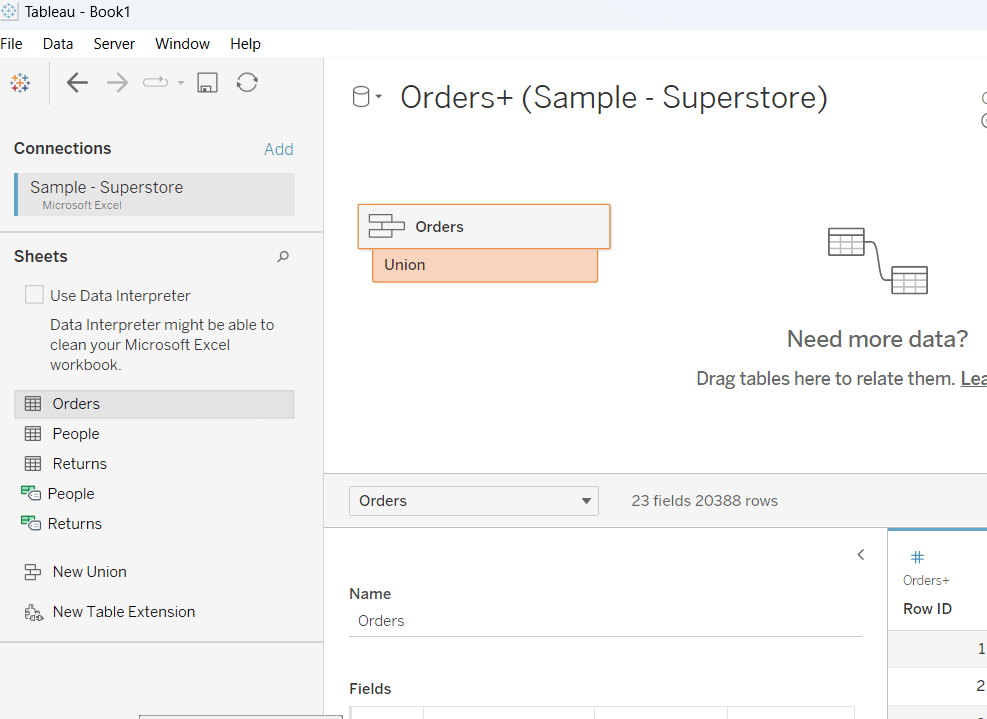
It was Yoshi’s turn to set the challenge this week. The requirement was to build a waterfall chart, and I have to confess I did end up having to have a sneak peak at Yoshi’s solution to point me in the right direction.

I tend to always be looking for generic solutions, and in this case trying to make use of Measure Names / Measure Values, but struggled to do this. When I peaked at the solution, I found there was an element of ‘hardcoding’ being applied for the specific layout. Armed with that knowledge, I was then able to build a solution which ended up differing from Yoshi’s, but (looks to) produces the same outcome.

Defining the reporting period

The viz is driven by a Base Date input control that allows the user to select a date. Based on the date selected, the viz then displays information for the whole of the previous month, and compares that to the same month in the previous year. This means if the user selects any date from 01 Aug 2025 to 31 Aug 2025, the viz shows the information related to the whole of July 2025 and compares it to July 2024.

We will use a parameter to capture the date inputted by the user, but rather than ‘hardcode’ the data to use, I’m going to set it based on a field in the data set that I’ll create

Date Default

IIF(YEAR(TODAY())>2025, #2026-01-01#, TODAY())

The data set we’re using goes up to 31 Dec 2025. To ensure the viz still shows data if it’s accessed in 2026 or beyond, I’m going to set the date to 01 Jan 2026 if we’re looking at the viz in 2026 or later, otherwise I’ll default to whatever ‘today’ may be. This means that from 01 Jan 2026 onwards, the viz by default will always show the data for December 2025 compared to December 2024.

With this field, I can then create the parameter

pDate

Date parameter that references the Date Default field when the workbook is first opened

And with the date captured by the user, we can then determine the date of the previous month we’ll be reporting over

Date – Last Month

DATE(DATEADD(‘month’, -1, DATETRUNC(‘month’, [pDate])))

This truncates the pDate value to the 1st day of that month, then subtracts a month to return the 1st day of the previous month. Eg if pDate is 20 Aug 2025, it is first truncated to 1st Aug 2025, then 1 month is subtracted to return 1st July 2025.

We’ll then refer to this field when determining all the measures we need to build.

Calculating the measures

There are multiple measures we need to determine to build this viz – information for the previous month, the previous month last year and then the difference between the two. So what follows is just a list of all these 🙂

Sales – Last Month

IIF(DATETRUNC(‘month’, [Order Date]) = [Date – Last Month], [Sales], NULL)

format this to $ with 0 dp.

Sales – Last Month LY

IIF(DATETRUNC(‘month’, [Order Date]) = DATEADD(‘year’,-1,[Date – Last Month]), [Sales], NULL)

format this to $ with 0 dp.

Sales – Last Month YoY

(SUM([Sales – Last Month]) – SUM([Sales – Last Month LY])) / SUM([Sales – Last Month LY])

custom format this to a % with 0 dp with an explicit + or – prefix : +0.0%;-0.0%;0.0%

Profit – Last Month

IIF(DATETRUNC(‘month’, [Order Date]) = [Date – Last Month], [Profit], NULL)

format this to $ with 0 dp.

Profit – Last Month LY

IIF(DATETRUNC(‘month’, [Order Date]) = DATEADD(‘year’,-1,[Date – Last Month]), [Profit], NULL)

format this to $ with 0 dp.

Profit – Last Month YoY

(SUM([Profit – Last Month]) – SUM([Profit – Last Month LY])) / SUM([Profit – Last Month LY])

custom format this to a % with 0 dp with an explicit + or – prefix : +0.0%;-0.0%;0.0%

Profit Margin – Last Month

SUM([Profit – Last Month])/SUM([Sales – Last Month])

format to % with 1 dp

Profit Margin – Last Month LY

SUM([Profit – Last Month LY])/SUM([Sales – Last Month LY])

format to % with 1 dp

Profit Margin – Last Month YoY

[Profit Margin – Last Month] – [Profit Margin – Last Month LY]

custom format this to a % with 0 dp with an explicit + or – prefix : +0.0%;-0.0%;0.0%

List Price

[Sales]/(1-[Discount])

List Price – Last Month

IIF(DATETRUNC(‘month’, [Order Date]) = [Date – Last Month], [List Price], NULL)

format to $ with 0 dp

List Price – Last Month LY

IIF(DATETRUNC(‘month’, [Order Date]) = DATEADD(‘year’,-1,[Date – Last Month]), [List Price], NULL)

List Price – Last Month YoY

SUM([List Price – Last Month]) – SUM([List Price – Last Month LY])

Discount Amount

[List Price] * [Discount]

Discount – Last Month

IIF(DATETRUNC(‘month’, [Order Date]) = [Date – Last Month], [Discount Amount], NULL)

Discount – Last Month LY

IIF(DATETRUNC(‘month’, [Order Date]) = DATEADD(‘year’,-1,[Date – Last Month]), [Discount Amount], NULL)

Discount – Last Month YoY

SUM([Discount – Last Month]) – SUM([Discount – Last Month LY])

Cost

[Sales]-[Profit]

Cost – Last Month

IIF(DATETRUNC(‘month’, [Order Date]) = [Date – Last Month], [Cost], NULL)

Cost – Last Month LY

IIF(DATETRUNC(‘month’, [Order Date]) = DATEADD(‘year’,-1,[Date – Last Month]), [Cost], NULL)

Cost – Last Month YoY

SUM([Cost – Last Month]) – SUM([Cost – Last Month LY])

There are additional fields we’ll need, but we’ll define these at the point we need them, as it’ll make more sense.

Building the KPIs

On a new sheet, double click into the Columns shelf and manually type MIN(0) to create a ‘fake axis’. Repeat this 2 more times, so 3 instances of MIN(0) exist and 3 marks cards exist. These are the placeholders for each of the KPIs we need to display.

On the 1st MIN(0) marks card, add Profit-Last Month and Profit – Last Month YoY to Label. Widen the row so you can see the text and change the mark type explicitly to Text. Adjust the label wording, layout and formatting as required, but don’t adjust the font colour. Instead create a new field

Colour – Profit

[Profit – Last Month YoY]>=0

and add this to the Colour shelf and adjust accordingly. Note – you will only ever get a true or false displayed and never both. You will need to adjust the date parameter to find a time period when the value is the opposite in order to set the opposite colour value.

Hide the Tooltip.

Repeat the process, adding Sales – Last Month and Sales – Last Month YoY to the 2nd MIN(0) marks card. Create

Colour – Sales

[Sales – Last Month YoY]>=0

and add to the Colour shelf.

The add Profit Margin – Last Month and Profit Margin – Last Month YoY to the 3rd MIN(0) marks card. Create

Colour – Profit Margin

[Profit Margin – Last Month YoY]>=0

and add to the Colour shelf. Hide column & row dividers, and name the sheet KPIs or similar.

Building the Waterfall

As mentioned above, this Waterfall chart involves a bit more “hardcoding” and the ‘explicit placement’ of the various measures into the viz.

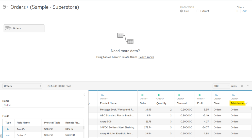
We are displaying 5 different measures, each one in a ‘specific column’. We’re going to make use of the Row ID field to define what measure is displayed where and how it will be formatted.

Add Row ID to the Dimensions pane (drag above the line in the data pane, so it is above Measure Names). On a new sheet, add Row ID to Filter and filter to rows 1-5 only. Then add Row ID to Columns. Create a new field

Header

CASE [Row ID]
WHEN 1 THEN ‘Profit (LY)’
WHEN 2 THEN ‘List Price Sales YoY’
WHEN 3 THEN ‘Total Discount’
WHEN 4 THEN ‘Total Cost YoY’
WHEN 5 THEN ‘Profit (TY)’
END

add this to Columns. Set the sheet to Fit Width.

This gives the start of the structure. We now want to display the relevant measure in each column, but we need a single field to do this, and the values of the fields need to be cumulative based on the preceding values.

Display Value

CASE [Row ID]
WHEN 1 THEN {FIXED: SUM([Profit – Last Month LY])}
WHEN 2 THEN {FIXED:SUM([Profit – Last Month LY])} + {FIXED:([List Price – Last Month YoY])}
WHEN 3 THEN {FIXED:SUM([Profit – Last Month LY])} + {FIXED:([List Price – Last Month YoY])} + (-1*{FIXED:[Discount – Last Month YoY]})
WHEN 4 THEN {FIXED:SUM([Profit – Last Month LY])} + {FIXED:([List Price – Last Month YoY])} + (-1*{FIXED:[Discount – Last Month YoY]}) – {FIXED: [Cost – Last Month YoY]}
WHEN 5 THEN {FIXED: SUM([Profit – Last Month])}
END

Here, we’re using a FIXED LoD calculation to ensure the measures we need are calculating across the whole data set and not segmented by the Row ID which we’re just using as an arbitrary placeholder.

Add this to Rows and change the mark type to gantt bar.

The size of the gantt bar is determined by the specific measures (rather than the cumulative values)

Size

(CASE [Row ID]
WHEN 1 THEN {FIXED: SUM([Profit – Last Month LY])}
WHEN 2 THEN {FIXED:([List Price – Last Month YoY])}
WHEN 3 THEN (-1*{FIXED:[Discount – Last Month YoY]})
WHEN 4 THEN -1*{FIXED: [Cost – Last Month YoY]}
WHEN 5 THEN {FIXED: SUM([Profit – Last Month])}
END) -1

Add this to Size

To label the bars create

Label

ABS([Size])

format this to $ with 0 dp. Add to Label and align centrally.

For the colouring create

Colour

IF ([Row ID]) = 1 THEN ‘Light’
ELSEIF ([Row ID]) = 5 THEN ‘Dark’
ELSEIF -1 * [Size] > 0 THEN ‘Blue’
ELSE ‘Red’
END

and add to Colour and adjust accordingly. And then create

Label Indicator

IF [Row ID] = 2 AND [Colour]= ‘Blue’ THEN ‘+’
ELSEIF (([Row ID] =3) OR ([Row ID]) = 4) THEN
IF [Colour]=’Blue’ THEN ‘-‘
ELSE ‘+’
END
END

Add to Label and adjust the font and layout of the label text accordingly.

Tidy up the formatting by

  • Adjust font style of the Header label.
  • Hide the Row ID pill (uncheck show header)
  • Hide the ‘header’ label (right click > hide field labels for columns)
  • Hide the axis title
  • Adjust the font style of the axis
  • Hide all axis lines/zero line, row & column dividers
  • Adjust the Tooltip
  • Name the sheet Waterfall or similar

Add the two sheets onto a dashboard and arrange with the parameter as required.

My published viz is here.

Happy Vizzin’!

Donna

Can you build a scatterbox?

I’m back from my holibobs, so back to solving #WOW2023 challenges and writing up the solutions – it’s tough to get back into things after a couple of weeks of sunshine and cocktails!

Anyway, this week, Sean set this challenge from Felicia Styler to build a scatterplot / heat map combo chart, affectionally termed the ‘scatterbox’.

Phew! This took some thinking… I certainly wasn’t gently eased back into a challenge!

Modelling the data

We were given a hint that the data needed to be unioned to build this viz. I connected to the Sample-Superstore.xls file shipped with 2023.2 instance of Tableau Desktop. After adding the Orders sheet to the canvas, I then added another instance, dragging the second instance until the Union option appeared to drop it on.

The union basically means the rows in the Orders data set are all duplicated, but an additional column called Table Name gets automatically added

This field contains the value Orders and Orders1 which provides the distinction between the duplicated fields caused by the union. It is this field that will be used to determine which data is used to build the scatter plot and which to build the heat map.

Building out the calculated fields

Let’s start just by seeing how the data looks with the measures we care about.

Onto a sheet add Product ID, Product Name and Table Name to Rows (Note – there are multiple Product Names with the same Product ID, so I’m treating the combination as a unique product). Then add Quantity to Text. The drag Discount and drop onto the table when it says ‘Show Me’, which should automatically add Measure Name/Measure Values into the view. Aggregate Discount to AVG. We can see that we’re getting the same values for each Table Name, which is expected.

When plotting the scatter plot, we’re plotting at the Product level, so the values above is what we’ll want to plot. But when building the heatmap, we need to ‘bin’ the values.

For the Quantity, we’re grouping into bins of size 10, where if the Quantity is from 0-9 the bin value is 0, 10-19, the bin value is 10 etc.

Quantity Bin

FLOOR({FIXED [Product ID], [Product Name], [Table Name]: SUM([Quantity])}/10) * 10

The LoD (the bit between the {} is returning the same values listed above, but we’re using an LoD, as when we build the heat map, we don’t want the Product fields in the view, but we need to calculate the Quantity values at the product level (ie at a lower level of detail than the view we’ll build). Dividing the value by 10, then allows us to get the FLOOR value, which ’rounds’ the value to the integer of equal or lesser value (ie with FLOOR, 0.9 rounds to 0 rather than 1). Then the result is re-multiplied by 10 to get the bin value.

So if the Quantity is 9, dividing by 10 returns 0.9. Taking the FLOOR of 0.9 gives us 0. Multiplying by 10 returns 0.

But if the Quantity is 27, dividing by 10 returns 2.7. The FLOOR of 2.7 is 2, which when multiplied by 10 is 20.

We apply a similar technique for the Discount bins, which are binned into groups of 0.1 instead.

Discount Bin

FLOOR({FIXED [Product ID], [Product Name], [Table Name]: AVG(Discount)}*10) / 10

Add these into the table to sense check the results are as expected.

Next we’re going to determine the values we want based on whether we’re building the scatter or the heat map.

Qty – Scatter

IF [Table Name] = ‘Orders’ THEN {FIXED [Product ID], [Product Name], [Table Name]: SUM([Quantity])} END

ie only return the Quantity value for the data from the Orders table and nothing for the data from the Orders1 table.

Qty – Heatmap

IF [Table Name] = ‘Orders1’ THEN [Quantity Bin] + 5 END

so, this time, we’re only returning data for the Orders1 table and nothing for the Orders table. But we’re also adjusting the value by 5. This is because by default, when using the square mark type which we’ll use for the heatmap, the centre of the square is positioned at the plot point. So if the square is plotted at 10, the vertical edges of the square will be above and below 10. However, we need the square to be centred between the bin range points, so we shift the plot point by half of the bin size (ie 5).

Adding these into the table, and aggregating to AVG we can see how these values are behaving.

As we’re building a dual axis, one of the axis will need to be combined within a single measure, so we create

Qty to Plot

IF ([Table Name]) = ‘Orders’ THEN ([Qty – Scatter]) ELSE ([Qty – Heatmap]) END

Now we move onto the Discount values, which we apply similar logic to

Discount – Scatter

IF [Table Name] = ‘Orders’ THEN {FIXED [Product ID], [Product Name],[Table Name]: AVG([Discount])} END

Discount – Heatmap

IF [Table Name] = ‘Orders1’ THEN [Discount Bin] + 0.05 END

We’ll need is to be able to compute the number of unique products to colour the heatmap by. As mentioned earlier, I’m determining a unique product based on the combination of Product Id and Product Name. To count these we first need

Product ID & Name

[Product ID] + ‘-‘ + [Product Name]

and then we can create

Count Products

COUNTD([Product ID & Name])

The final calculations we need are required for the heatmap tooltips and define the range of the bins.

Qty Range Min

[Qty To Plot] – 5

Qty Range Max

[Qty To Plot] + 5

Discount Range Min

[Discount – Heatmap] – 0.05

Discount Range Max

[Discount – Heatmap] + 0.05

Now we can build the viz

Building the Scatterbox

On a new sheet, add Qty to Plot to Columns and change to be a dimension (so not aggregated to SUM) and Discount – Scatter (set to AVG) to Rows. Add Product ID and Product Name to Detail. Change the mark type to Circle and adjust the size. Adjust the Colour and reduce the opacity (I used #4a9aab at 50%)

Adjust the Tooltip.

Then add Discount – Heatmap to Rows. This creates a 2nd marks card. Change to be a dimension, and change the mark type to square. Remove Product ID and Product Name from the Detail shelf

Add Count Products to Colour and ensure the opacity is 100%. Adjust the sequential colour palette to suit and set the end of the range to be fixed to 300

Add Qty Range Min, Qty Range Max, Discount Range Min, Discount Range Max to the Tooltip shelf of the heatmap marks card. Set all to aggregate to AVG and adjust tooltip to suit.

Then make the chart dual axis and synchronise axis. Increase the size of the square heat map marks (note don’t worry how these look at this point, the layout will adjust when added to the dashboard. Right click on the Discount – Heatmap axis on the right and move marks to back. Hide that axis too.

Edit the Qty to Plot axis so the tick marks are fixed to increment every 10 units.

Adjust axis titles, remove row/column dividers and hide the null indicator.

Then add the sheet to an 800 by 800 sized dashboard. You will need to make tweaks to the padding and potentially sizing of the heat map marks again to get the squares to position centrally with white surround. I added inner padding of 60px to the left & right of the chart on the dashboard, to help make the chart itself squarer.

My published viz is here .

Happy vizzin’!

Donna

How many consecutive starts?

Another table calculation related challenge this week, set by Luke, visualising cumulative starts for NFL Quarterbacks per team from 2006.

Luke provided the data within a Tableau workbook template on Tableau Public, so I started by downloading the workbook and understanding the data structure.

The challenge talks about teams playing over 17 weeks, but the data showed some data associated to weeks 28-32. So I excluded these weeks by filtering them out.

I then started to build out the data in tabular form, so I could start to build up what was required. I added Team, Season, Week and Player ID to Rows, and just to reduce the amount of data I was working with while I built up the calcs, chose to filter to the Teams ARZ, ATL & BLT.

What we’re looking to do is examine each Player ID and work out whether it is the first record for the Team or whether it differs from the previous row’s data. If so then we’re at the ‘start’ of a run, so we record a ‘counter’ value of 1. If not, the values match, so we need to increment the counter.

We’ll do this in stages.

Firstly, let’s get the previous Player ID value.

Prev Player ID

LOOKUP(MIN([Player Id]),-1)

This ‘looks up’ the record in the previous (-1) row. Change this field to be discrete and add to the Rows. Set the table calculation to compute by all fields except Team.

Each Prev Player ID value matches the Player ID from the row before, unless its the first row for a new Team in which case the value is Null.

Then we can create a field to check if the values match

Match Prev Player ID

MIN([Player Id])=[Prev Player ID]

Add this to the view and set the table calc as above, and the data shows True, False or NULL

Now we can work out the consecutive streak values

Consecutive Streak

IF (NOT([Match Prev Player ID])) OR ISNULL([Match Prev Player ID]) THEN 1
ELSE 1+PREVIOUS_VALUE(-1)
END

If we don’t match the previous value or we’re at the start of a new team (as value is NULL), then start the streak by setting the counter to 1, otherwise increment the counter. Add this to the view and set the table calc for both the nested calculations as per the settings described above.

Next we need to identify the last value of the Consecutive Streak for each Team.

Current Streak

WINDOW_MAX(IF LAST()=0 THEN [Consecutive Streak] END)

The inner IF statement, will return the value of Consecutive Streak stored against the last row for the Team. All other rows will be Null/blank. The WINDOW_MAX() statement then ‘spreads’ this value across all the rows for the Team.

Add this onto the view, and set the table calc for all the nested calcs.

Finally, we need one more bit of data. The chart essentially plots values from 2006 week 1 through to 2020 week 17. We need to ‘index’ these values, so we have a continuous week number value from the 1st week. We can use the Index table calculation for this

Index

INDEX()

Add this field to the view, set it to be discrete (blue pill) and position after the Week field on the Rows. Set the table calc as usual, so the Index restarts at each Team.

Now we’ve got all the data points we need, we can build the viz. I did this by duplicating the tabular view and then

  • Remove Prev Player ID and Match Prev Player ID
  • Move Season, Week and Player ID from Rows to Detail
  • Move Current Streak from Text to Rows and change to be discrete (blue)
  • Move Index from Rows to Columns and change to be continuous (green)
  • Move Consecutive Streak from Text to Rows
  • Change mark type to bar, and set to fit width to expand the view.
  • Change Size to be Fixed, width size 1 and aligned right
  • Set the border on the Colour shelf to be None.
  • Remove the Team filter and adjust the row height

All that’s left now is to set the tooltip (add Player to the Tooltip shelf to help this), and then apply the formatting. You can use workbook formatting (Format -> Workbook menu) to set all the font to Times New Roman.

Hopefully this is enough to get you to the end 🙂 My published viz is here.

Happy vizzin’! Stay Safe!

Donna

Is Profit Ratio Influenced by Quantity?

For this week’s challenge, Ann asked we recreated a scatter plot that ‘on click’ became a connected scatter plot and also displayed an ‘insights’ box to the user.

Building out the data

The scatter plot is to show Profit Ratio by Quantity, so first up we need

Profit Ratio

SUM([Profit])/SUM([Sales])

formatted to percentage with 0 dp.

A mark is shown on the scatter plot per Category and Month/Year. When working with dates like this, I often prefer to created a dedicated field to use as an ‘exact date’ which I can then format. So I built

Month Year

DATE(DATETRUNC(‘month’,[Order Date]))

and formatted it to the March 2001 format (ie mmmm yyyy).

We’re also going to need a set based on the Category field, as that is going to drive the interactivity to help us connect the dots ‘on click’. So right click on Category and Create Set and just tick one of the categories displayed for now.

Selected Category

Let’s build these out into a table as follows

  • Order Date to Filter, filtered by years 2018 & 2019
  • Category, Selected Category & Month Year (exact date , discrete) onto Rows
  • Measure Names to Text and Filter to Quantity & Profit Ratio
  • Right click on Selected Category and select Show Set to display a selection control to easily allow the set values to be changed

To help drive the interactivity, we’re going to need to store the value of the Profit Ratio for the Selected Category in the set.

Selected PR

IF ATTR([Selected Category]) THEN [Profit Ratio] END

Format this to percentage 0 dp too, and add this to the table – it will only display the profit ratio against the rows associated to the category in the set

At this point, we’ve got what we need to build out the scatter plot, but I’m going to continue to create the fields needed for the ‘Insights’ piece.

These are looking for the months that contained the Max & Min values for the Profit Ratio and Quantity. I’m going to tackle this with Table Calcs.

Max PR per Category

WINDOW_MAX([Profit Ratio])

Adding this to the table, and setting the table calculation to compute by Month Year only, gives us the Max Profit Ratio for each Category

We need 3 more fields like this :

Max Qty per Category

WINDOW_MAX(SUM([Quantity]))

Min PR per Category

WINDOW_MIN([Profit Ratio])

Min Qty per Category

WINDOW_MIN(SUM([Quantity]))

Add all these to the table, setting the table calc in the same way as described above.

Now we know what the min & max values are, we need to know the month when these occurred.

Max PR Month

WINDOW_MAX(IF ATTR([Selected Category]) AND [Profit Ratio] = [Max PR per Category] THEN MIN([Month Year]) END)

Format this to March 2001 format.

If the category is that selected, and the profit ratio matches the maximum value, then retrieve the Month Year value, and duplicate that value across all the rows (this is what the outer WINDOW_MAX does).

Add this to the table in the Rows, and adjust the table calc settings for both the nested calculations to compute by Month Year only. The month for the selected category which had the highest profit ratio will be displayed against all rows for that category, and null for all other rows.

Again we need similar fields for the other months

Max Qty Month

WINDOW_MAX(IF ATTR([Selected Category]) AND SUM([Quantity]) = [Max Qty per Category] THEN MIN([Month Year]) END)

Min PR Month

WINDOW_MAX(IF ATTR([Selected Category]) AND [Profit Ratio] = [Min PR per Category] THEN MIN([Month Year]) END)

Min Qty Month

WINDOW_MAX(IF ATTR([Selected Category]) AND SUM([Quantity]) = [Min Qty per Category] THEN MIN([Month Year]) END)

Format all these too, and add to the table with the appropriate table calc settings applied.

If you now change the value in the the Selected Category set, you should see the table update.

Building the Scatter Plot

On a new sheet, build out the basic scatter plot by

  • Order Date to Filter, filtered by years 2018 & 2019
  • Profit Ratio to Rows
  • Quantity to Columns
  • Category to Colour and adjust accordingly
  • Month Year exact date, continuous to Detail
  • Change Shape to filled circle
  • Adjust the Tooltip to suit
  • Change the axis titles to be capitalised
  • Change the sheet title
  • Remove all row/column borders & gridlines. Leave the zero lines and set the axis rulers to be a sold grey line

Add Selected PR to Rows, and change the mark type of that card to line, and add Month Year to path. In the image below, I still have Furniture selected in my set.

Add Month Year to the Label shelf too and format so the text is smaller and coloured to match mark colour

Make the chart dual axis, synchronise the axis and remove the Measure Names from the colour shelf of each mark. Hide the Selected PR axis.

If you now change the selected set value, you can see how the other categories ‘join up’.

Building the Insights Box

Take a duplicate of the data table built originally, and add Selected Category to Filter. If you’ve still got an entry in your set, this should reduce the rows to just those records for that Category.

Remove the fields Profit Ratio, Quantity, Selected PR from the Measure Values section, and remove Selected Category from Rows.

Create a new field

Index = Size

INDEX()=SIZE()

and add this to the Filter shelf, setting the value to true.

The INDEX() function will number each row, the SIZE() function will number each row based on the total number of rows displayed (ie all rows will display the same number), so INDEX()=SIZE() will return true for the last row only

Now we’ve only got 1 row displayed, we’ve got the info we need to build the data in the Insights box by

  • Move Month Year to Detail
  • Category to Colour
  • Move Max PR Month, Max Qty Month, Min PR Month, Min Qty Month to Text
  • Move Max PR per Category, Max Qty per Category, Min PR Per Category, Min Qty per Category to Text

This will probably show duplicate instances of the values. This is because we didn’t fix the table calculation setting of the Index=Size field. Edit that to compute by Month Year

and then re-edit the Index=Size filter to just be true again, and expand the display so you can see all the values.

Now you can easily format the Text to the required display

I used this site to get the bullet point image from

Building the dashboard & interactivity

Add the scatter plot to the dashboard, and remove the legends that automatically get added.

Float the Insights sheet and position bottom right, remove the title. fit entire view, and also remove the colour legend which will have been added.

Add a dashboard Set Action to assign values to the Selected Category set and remove all values when the selection is cleared

Additionally, add a highlight action that highlights the Category field only (this keeps the lines highlighted on selection of a single mark).

Now practice clicking on and off marks on the scatter plot and you should see your lines & insights box being added and removed.

Finally add the title and header line by adding a vertical container at the top above the scatter plot.

Add a text box for the title, and underneath add a blank object.

Set the padding of the blank object to 0 and the background to black. Then edit the height to 4, and adjust the height of the container if it’s now too large.

Make adjustments to the position of the floating insights box if need be so it isn’t overlapping any axis.

And that should be it! My published viz is here.

I’ll be taking a break for a couple of weeks, so will be on catch up when I return from some R&R.

Happy vizzin’! Stay Safe!

Donna