Yoshi set this week’s challenge which focused on 2 areas : the use of tools such as CHAT GPT to help us create Tableau RegEx functions (which are always tricksy), and the build of the chart itself.
Creating the REGEX calculated fields
I chose to use CHATGPT and simply entered a prompt as
“give me a regex expression to use in Tableau which extracts a string from another string in a set format. The string to interrogate is”
and then I pasted in the string I’d copied from one of the Session Html fields. I got the following response
along with many more code snippet examples. I used these to create
returns the day of the session as a proper date field, all hardcoded to 2023, since this is when the data is from.
Start Date
DATETIME(STR([Date]) + ” ” + [Start Time])
returns the actual day & start time as a proper datetime field.
End Date
DATETIME(STR([Date]) + ” ” + [End Time])
Duration
DATEDIFF(‘second’, [Start Date], [End Date])
Add fields to a table as below
Firstly, when we build the viz, we’ll need to sort it based on the Start Date, the Session Level (where Advanced is listed first, and All Levels last) and the Duration (where longer sessions take higher precedence) . For this we need a new field which is a combination of information related to all these values.
Sort
STR([Start Date]) + ‘ – ‘ + STR( CASE [Session Level] WHEN ‘advanced’ THEN 4 WHEN ‘intermediate’ THEN 3 WHEN ‘beginner’ THEN 2 ELSE 1 END ) + STR([Duration]/100000)
(this just took some trial and error)
Add this to the table after the Session ID pill and then apply a Sort to the Session ID pill so it is sorting by the Minimum value of the field SortAscending. You should see that when the start time and session level match, the sessions are sorted with the higher duration first.
The viz also lists the AM & PM sessions as separate instances, where the 1st session of the PM session is displayed on the same ‘row’ as the 1st session of the AM session. To handle this we need
Session Index
INDEX()
Make this discrete and add to the table after the AM|PM pill. Change the table calculation so it is computing by all fields except AM|PM and Session Date. The numbering should restart at each am/pm timeslot
Finally, the last field we need to build this viz, is another date field, so we can position the gantt chart bars in the right places. As the viz already segments the chart by Session Date and AM|PM, we can’t reuse the existing Start Date field as this will display the information as if staggered across the 3 days. Instead we want to create a date field, where the day is the same for al the sessions, but just the time differs
Baseline Date
DATETIME(STR(#2023-01-01#) + ” ” + [Start Time])
the date 01 Jan 2023 is arbitrary and could be set to any day. Add this into the table, so you can see what it’s doing. You will probably need to adjust the table calculation on Session Index again to include Baseline Date in the list of checked fields.
Building the viz
On a new sheet, add Session Date to Columns and manually re-order so Tuesday listed first. Then add AM|PM to Columns . Add Baseline Date as a continuous exact date (green pill) to Columns . Add Session Id to Detail then add Session Index to Rows and adjust the table calculation so it is computing by all fields except Session Date and AM|PM.
Create a new field
Size
SUM([Duration])/86400
and add this to the Size shelf. 86400 is the number of seconds in 24hrs, so adjusts the size of the gantt bars to fit the timeframe we’re displaying.
Add Session Level to Colour and adjust accordingly. You will need to readjust the Session Index table calc to include Session Level in the checked fields. Add a border to the bars. Edit the Baseline Date axis so the axis ranges are independent
Add Description and Session Title to Detail and again adjust the Session Index table calc to include these fields too. Apply a Sort to the Session Id field so the data is sorted by the Sort field descending
Add Location, Start Time and End Time to Tooltip, and update accordingly. Then apply formatting to
change font of the Session Date and AM|PM header values
remove the Session Date/ AM|PM column heading label (right click > hide field labels for columns)
Hide the Session Index field
Hide the Baseline Date axis
Add column banding so the Wednesday pane is coloured differently
Add the ability to highlight the Session Title and Description by selecting Show Highlighter from the context menu of each pill
Then add the sheet to a dashboard, using containers to display the colour legend and the highlighter fields.
It’s back to the EFL this week for my #WOW challenge. Once again I’ve tried to provide a multi-level challenge – a version that uses some core skills and features, and a version that just pushes the display a bit further, just for fun. I’ll start with the core build and then use that as the base for the bonus challenge.
Setting up the parameters
The main crux of this challenge is measure swapping, so for this we need a parameter
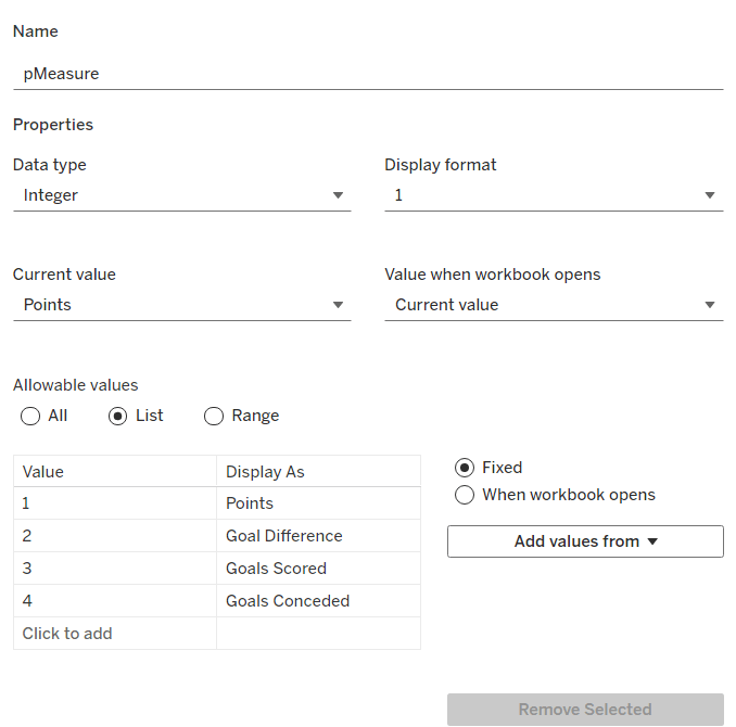
pMeasure
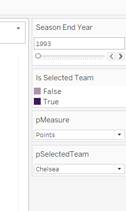
integer parameter listing values 1 to 4 which are aliased as per the screen shot below. Default value is 1 (Points).
Note – you can use a string parameter with the actual words. I just chose to use this method to demonstrate the aliasing ability. Also when referencing this parameter in a CASE statement (which we’ll do shortly), using integer values for comparisons is slightly more efficient than string comparisons.
We also need the user to have the ability to select the team they want to track
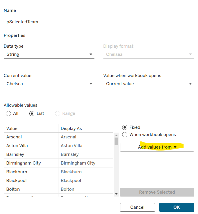
pSelectedTeam
string parameter defaulted to your preferred team (I chose Chelsea). This is a List parameter that is populated from the Team field via the Add values from button
Building the calculations
We need to determine the measure to display based on the parameter selection
Measure to Display
CASE [pMeasure] WHEN 1 THEN SUM([Cumulative Points]) WHEN 2 THEN SUM([Cumulative Goal Difference]) WHEn 3 THEN SUM([Cumulative Goals For]) WHEN 4 THEN SUM([Cumulative Goals Against]) END
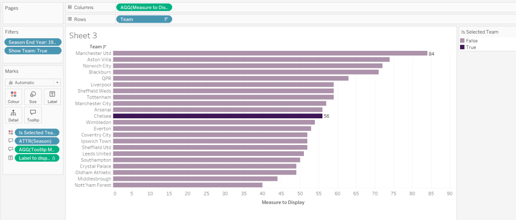
We also will need to colour the bars based on the selected team
Is Selected Team
[Team]=[pSelectedTeam]
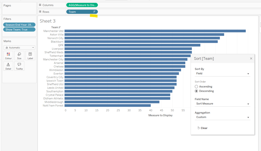
and we need to sort the data based on best to worst, but need to consider that for Goals Conceded, the higher the value the worse the team is.
Sort Measure
IF [pMeasure] = 4 THEN [Measure to Display]*-1 ELSE [Measure to Display] END
We only want to show teams once they start participating in a Season. For this, we need to identify the team’s 1st season in the EFL
1st Season per Team
{FIXED [Team]: MIN(IF [Cumulative Points] > 0 THEN [Season End Year] END)}
and then we can create a field we can filter on, based on this
Show Team
[Season End Year]>=[1st Season per Team]
We only want to show a label against the 1st team and the selected team, so create
Label to display
IF MIN([Is Selected Team]) OR FIRST()=0 THEN [Measure to Display] END
and finally, we need to display the value of the current season’s measure on the tooltip, as well as the cumulative value, so we need another case statement
Tootltip Measure
CASE [pMeasure] WHEN 1 THEN SUM([Points]) WHEN 2 THEN SUM([Goal Difference]) WHEn 3 THEN SUM([Goals For]) WHEN 4 THEN SUM([Goals Against]) END
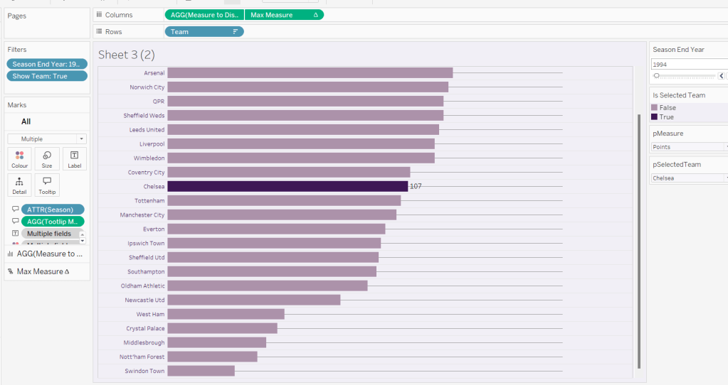
Building the core bar chart
On a new sheet, add Team to Rows and Measure to Display to Columns. Add Season End Year to Filter and select 1993. Add Show Team to Filter and select True. Apply a sort to the Team field to sort by the field Sort Measure descending.
Add Is Selected Team to Colour and adjust accordingly. Add Label to display to Label. Add Season and Tooltip Measure to Tooltip and update accordingly,
Show the pMeasure and pSelectedTeam parameters and the Season End Year Filter. Adjust the Season End Year filter control so that the All option isn’t available and it displays as a single value slider control.
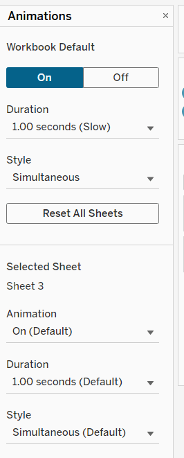
Move the Season End Year filter control on by one value and notice how the chart transitions. Adjust the Animations settings (Format menu > Animations) to be sequential and slow
Finally tidy up the display by
hiding the Measure to Display axis (right click > uncheck show header)
hiding the Team row label (right click > hide field labels for rows)
widen each row a bit
hide gridlines, zero lines, axis rulers and axis ticks
add pale grey row dividers
set the background colour of the worksheet
adjust the font of the row labels – I used Tableau Book 8pt in colour #3e1756 (dark purple)
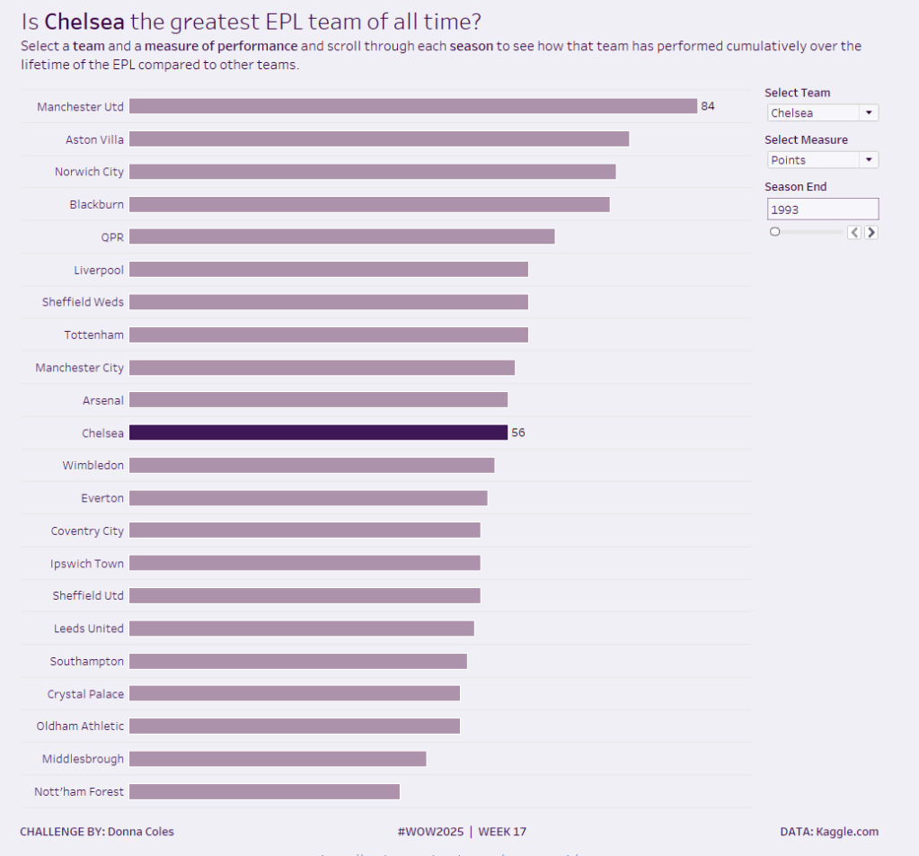
Name the sheet Core or similar and add to a dashboard setting it to Fit Entire View
Add a title to the dashboard that references the pSelectedTeam parameter.
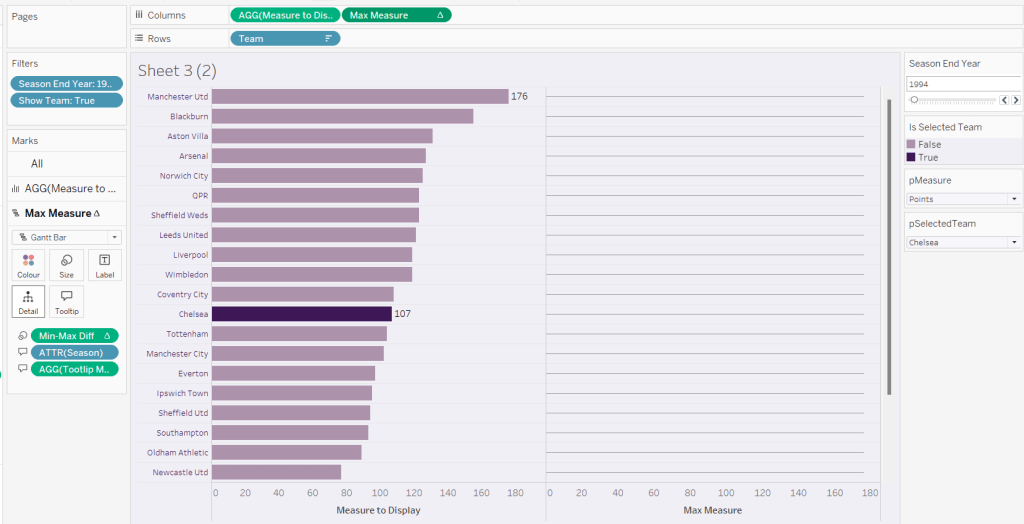
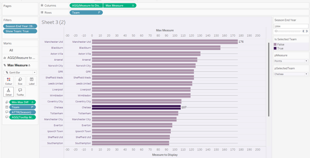
We’re going to use a gantt bar to simulate a central line for each row. This bar needs to extend to the largest measure in the table for every row, so this is the point we’ll plt
Max Measure
WINDOW_MAX([Measure to Display])
Add this to the Columns shelf, and on the Ma Measure markls card that gets added, remove the Is Selected Team from the Colour shelf, and change the mark type to gantt bar.
The bar needs to extend to the 0 or the minimum value in the window (if its less than 0), so we need a field to show the difference between the max and the minimum of 0 or the ‘window min’, but we need to multiple by -1 so the size extends in the right direction.
Max-Min Diff
([Max Measure] – MIN(WINDOW_MIN([Measure to Display]),0)) * -1
Add this to the Size shelf, and then update the size to be as small as possible. Remove Label to Display from the marks card and add a border the same colour as the background to the Gantt bar (via the Colour shelf) to make the line very narrow.
Add Team to the Label shelf and align centre left. Format the label text to be 8pt and dark purple. Then make the chart dual axis and synchronise the axis.
Right click the top axis and select move marks to back. Then hide both axis (right click, uncheck show header) and hide the Team pill on Rows too (again uncheck show header)
Verify the Tooltip on the gantt bar displays the same as on the main bar. If not add the relevant fields and adjust to match.
Tidy up the formatting by removing the row and column dividers. If need be adjust the colour of the Gantt bar to be a paler grey.
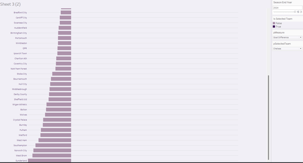
Change the measure value to Goal Difference and adjust the year to 2024 and check the display looks as expected, especially at the bottom – the gap between the label of the team at the bottom and the bar is minimal.
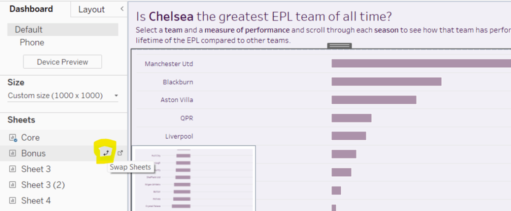
Add the chart to a dashboard – the simplest way is to duplicate the core dashboard and then use the swap sheets feature to quickly swap the main vizzes.
Community month continues this week with Yama G posing us this challenge to analyse profit ratio.
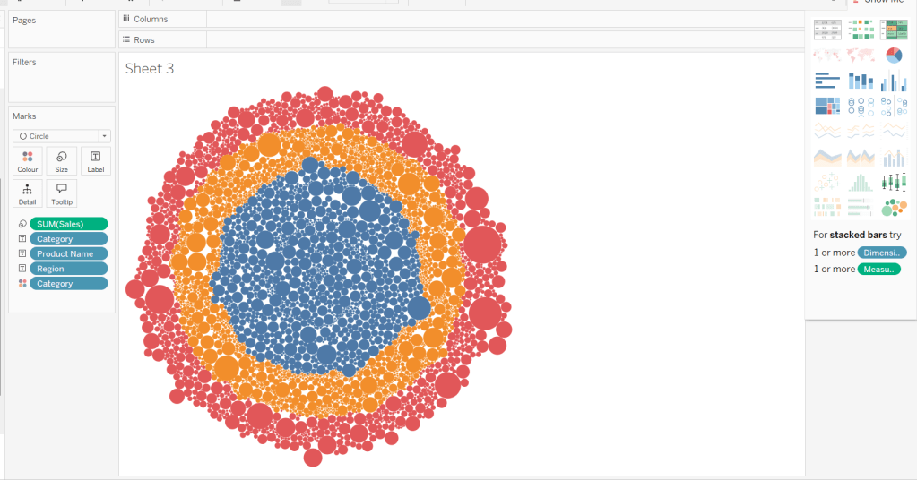
Building the basic bubble chart
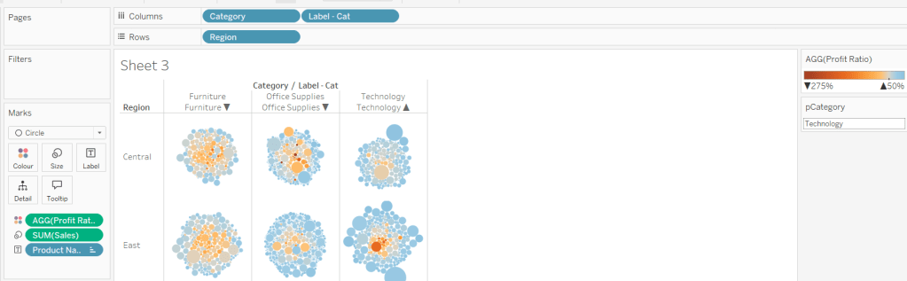
The simplest way I found to start this, was to use ctl-click to multi-select Category, Region, Product Name and Sales from the data pane, and then select the packed bubbles option from the Show Me menu.
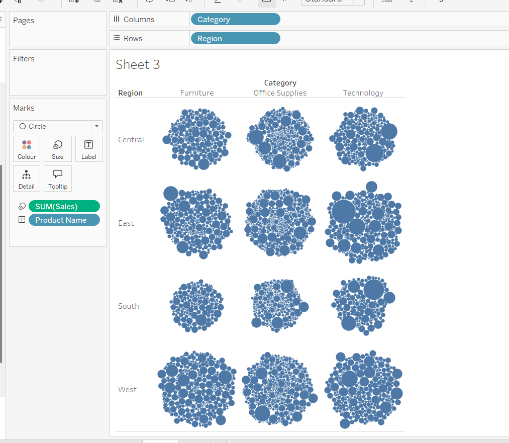
Then move Category from Text to Columns and Region from Text to Rows, and remove Category from Colour.
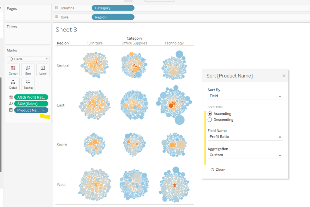
Create a new field
Profit Ratio
SUM(Profit)/SUM([Sales])
and apply a custom number format of 0%;▲0%;0% (in this instance I think the intention is to use the ▲ as ‘warning’ indicator).
Add this to Colour. To cluster the lower profit ratios towards the centre of the bubbles, add a sort to the Product Name pill on the Text shelf, to sort ascending by Profit Ratio.
Note – you can’t influence quite how the bubbles are arranged, so it’s possible the layout you see may differ slightly from the solution.
Showing details for selected Sub-Category
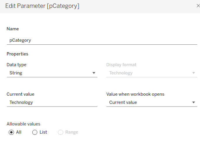
Clicking on a Category in the bubble viz should expand to show the Sub-Categories. To support this we need a parameter
pCategory
string parameter defaulted to Technology
The Category label displayed needs to show an arrow indicator based on whether the Category is selected or not
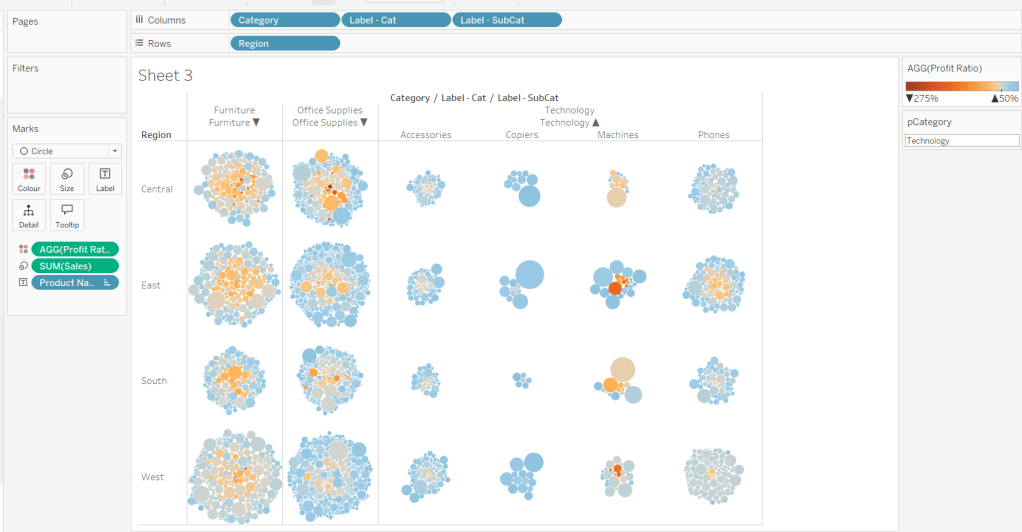
We want to show Sub-Category details for the selected Category, so create
Label – SubCat
IIF([pCategory]=[Category], [Sub-Category], ”)
Add this to Columns too.
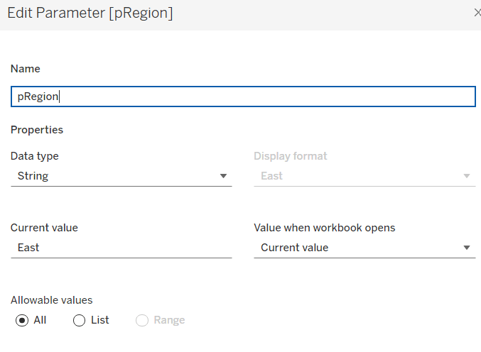
There is a need to capture the Region too, as part of the sorting on the tabular viz. But the Region header label needs to indicate the selected region. We will need a parameter
pRegion
string field defaulted to East
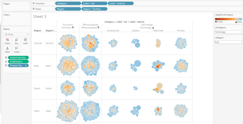
And then a new field
Region * Sortkey
[Region] + IIF([pRegion]=[Region],’*’,”)
Add this to Rows.
Finally tidy up by
adjusting the Tooltip
hide the Region pill (uncheck show header)
hide the Category pill (uncheck show header)
hide the Region * Sortkey row heading label (right click -> hide field labels for rows)
hide the Label – Cat / Label SubCat column heading label (right click -> hide field labels for columns)
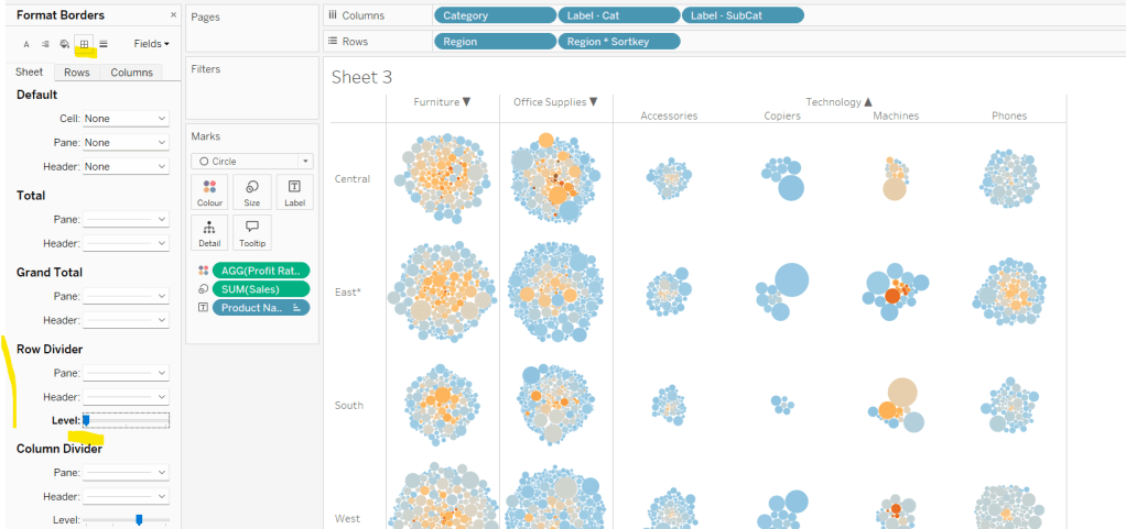
remove the row dividers in the body of the viz (set the Level to 0)
Update the sheet title and name the sheet Bubble or similar.
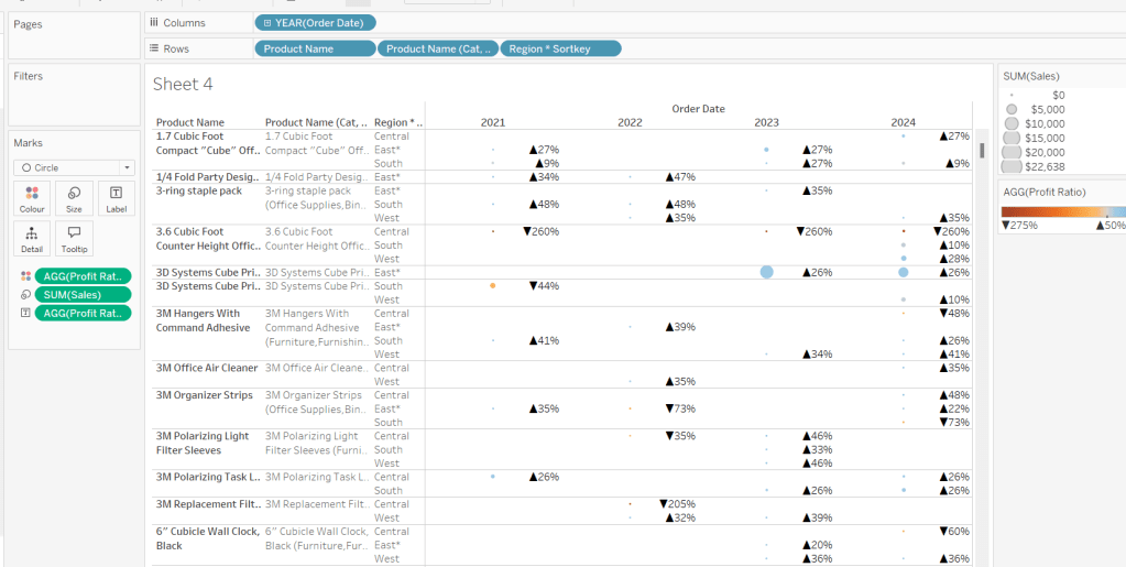
Building the basic Product Detail table
The first column is a combination of fields, so create
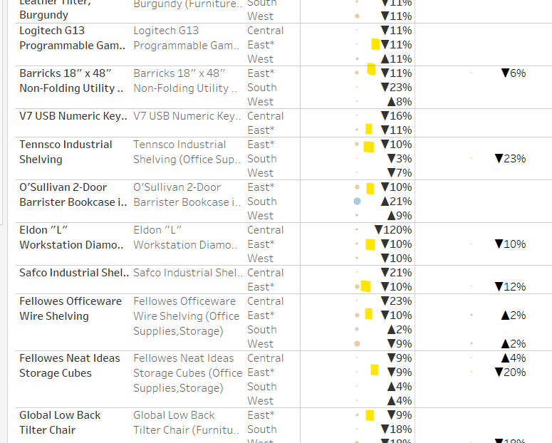
Add Product Name,Product Name (Cat, SubCat) and Region * Sortkey to Rows and Order Date as a discrete (blue) pill at the Year level to Columns. Change the mark type to circle. Add Sales to Size and Profit Ratio to Colour. Add Profit Ratio to Label and align right. Set the table to Fit Width. Increase the Size of the circles a bit.
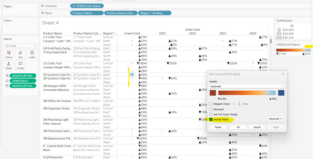
Add totals via Analysis > Totals > Show Row Grand Totals and then via the same menu, select the Row Totals to Left option. Edit the Colour Legend and select the Include Totals option, so the circles in the total column are also coloured.
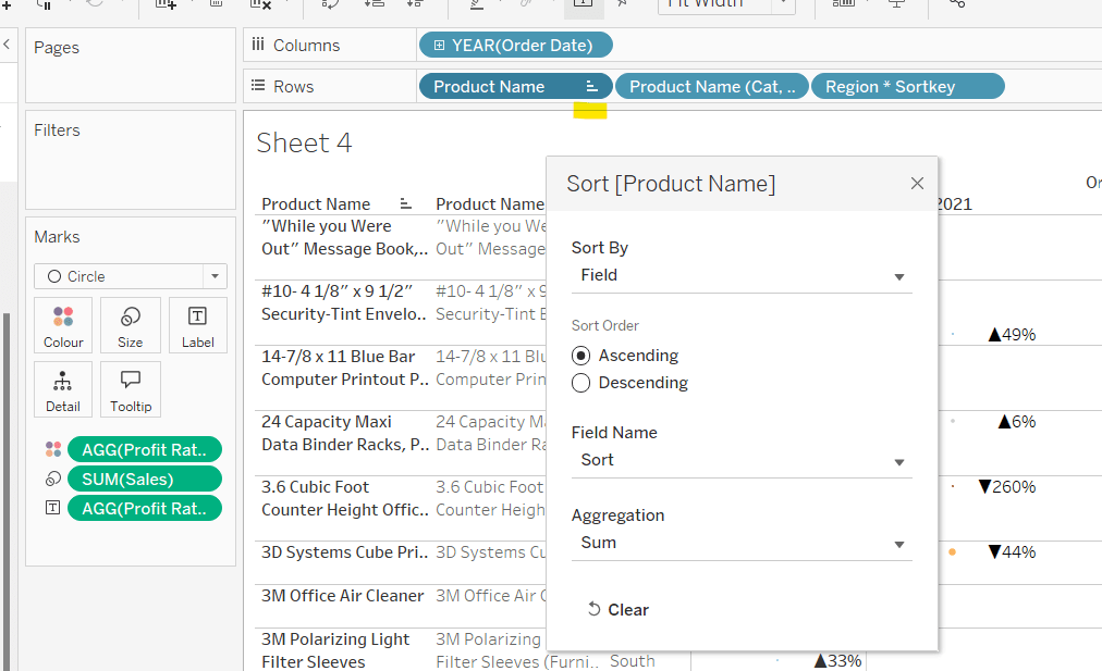
Applying the table sort
The requirement is to sort each Product Name based on the value of the Profit Ratio associated to the selected Region. The data should be sorted ascending.
This took me a little while to figure out – initially I wanted to use a table calculation, but you can’t apply a sort to a field based on that, and if you then add it as a discrete measure, you can’t have total columns. So I figured it out eventually. Firstly, I need to capture the Profit Ratio for each Product Name and Region (essentially the value listed in the Grand Total column). I can use an LOD for this.
but I then only want the value associated to the selected Region, and I want to ‘spread’ this across every row for the Product Name. So I can use another LOD but just at the Product Name level, which in turn uses a nested IF statement, to just return the value we care about.
Sort
{FIXED [Product Name]: AVG(IIF([Region]=[pRegion],[PR by Product & Region],NULL))}
Apply a Sort to the Product Name pill in Rows to sort by the field Sort ascending
You should find that when you see some Product Names that have sales in the selected region (in this case East), that the products are listed based on this value with the lowest Profit Ratio first (note the East row isn’t listed first if there are sales for the Central region, as the rows within each product are listed alphabetically based on the region name.
Finally tidy up by
Adjusting the Tooltip to suit
Hide the Product Name pill (right click, uncheck show header)
Adjusting the font style of the fields and label headings.
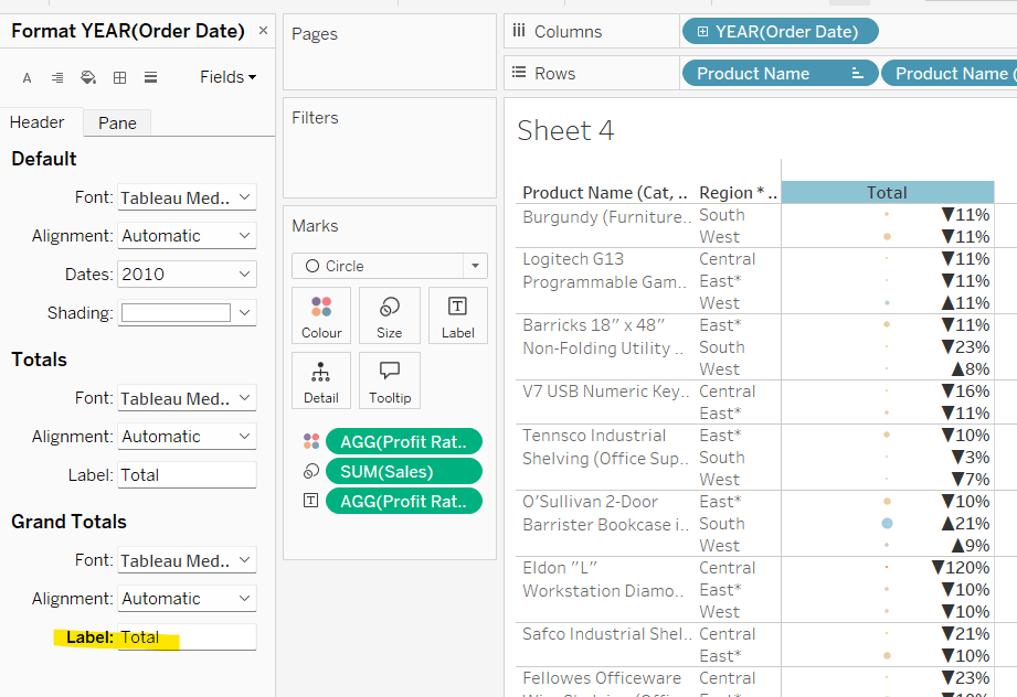
Rename the Grand Total label to Total (right click the label > format and update the Label value)
hide the Order Date column heading label (right click > hide field labels for columns)
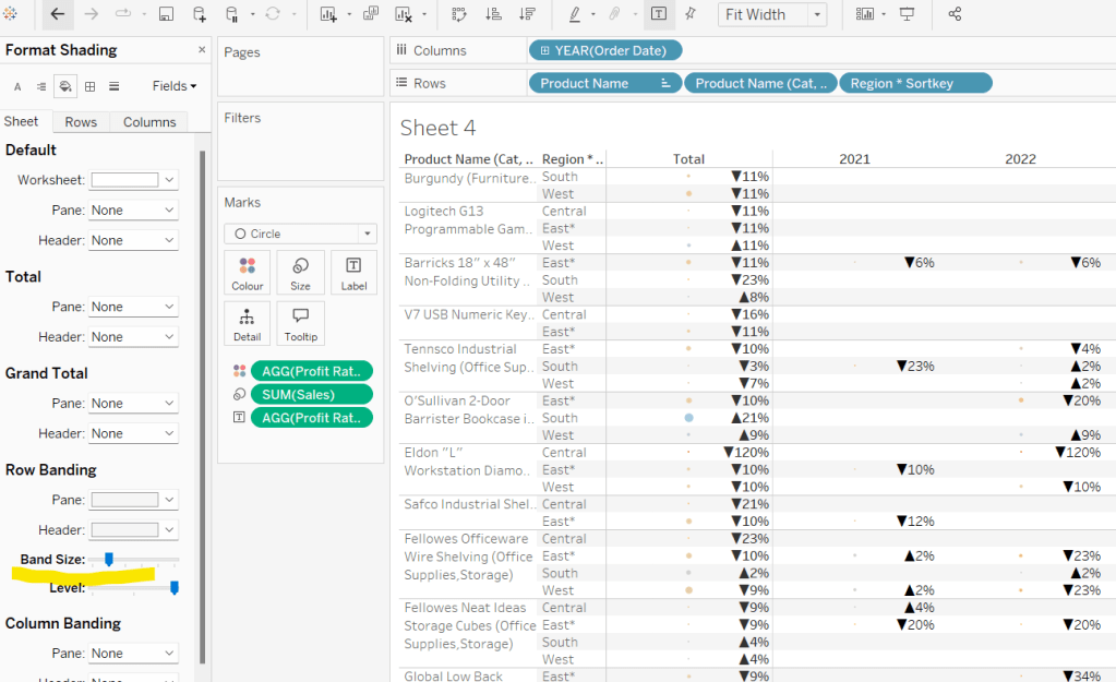
add row banding (right click viz to format), then adjust band size to level 1
Update the sheet title and name the sheet Table or similar.
Building the dashboard and adding the interactivity
Using layout containers, add the two sheets onto the dashboard, adding a title and the relevant legends (note I used text objects for the Profit Ratio legend title and the Sales ‘legend’.
We need several dashboard actions:
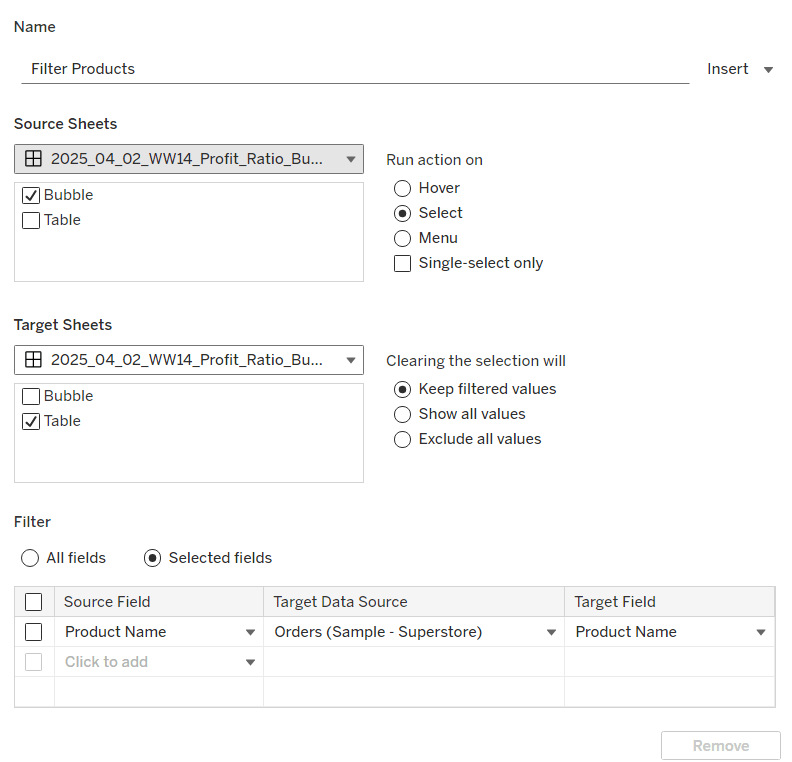
Filter Products
Dashboard filter action, that on select of the Bubble sheet, targets the Table sheet, passing through the Product Name only. The set of products is retained when the selection is cleared.
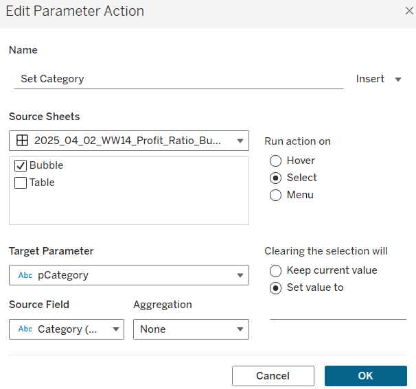
Set Category
Dashboard parameter action, that on select of the Bubble sheet, sets the pCategory parameter with the value from the Category field. When the selection is cleared, the parameter is reset to <empty string>
This action will allow the bubble chart to ‘expand and collapse’ on click.
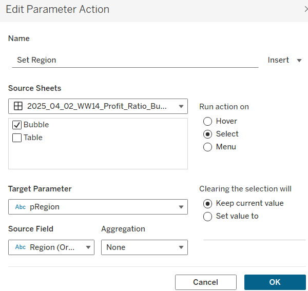
Set Region
Dashboard parameter action, that on select of the Bubble sheet, sets the pRegion parameter with the value from the Region field. When the selection is cleared, the parameter is retained
This action will apply the ‘niche’ sort and the relevant region labels will be updated with an * too.
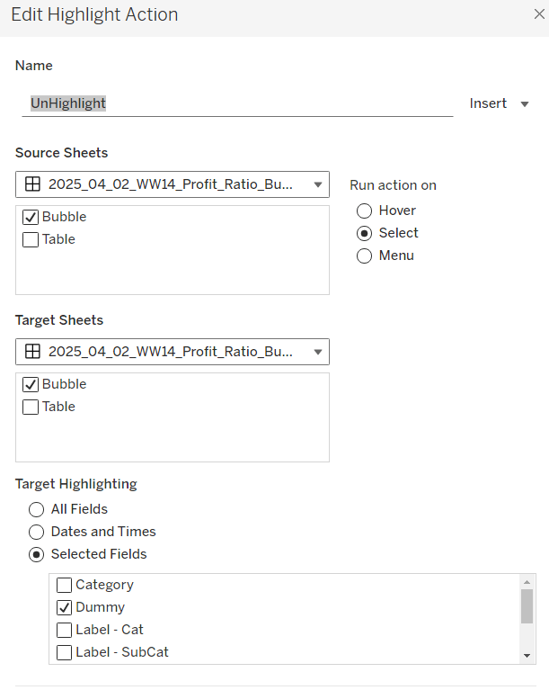
Finally, on selection of products in the bubble viz, we don’t want the other marks to ‘fade’ To stop this from happening, create a new field
Dummy
‘Dummy’
and add to the Detail shelf on the Bubble sheet.
Then add a dashboard highlight action
UnHighlight
On select of the Bubble sheet, target the Bubble sheet selecting the field Dummy only
And with that you should have a functioning dashboard. My published viz is here.
Note, after testing, I did notice a difference in the behaviour of my version to the solution. When I deselect all products from the bubble chart when in an expanded state, the section will collapse. The solution uses a ‘fake header’ sheet to stop this from happening, which is then carefully positioned above the bubble chart sheet. I’m ultimately happy with my 2-sheet solution, but feel free to check out the challenge solution for a better understanding.
Erica set the challenge this week, and I’m not gonna lie, I found this tough. On the face of it, it looks like something I felt I should be ok at, but nuances cropped up as I was building that meant I often had to change tact and try something different.
My intention was to build each version – Beginner, Intermediate then Advanced, adding to my solution each time, but decisions I made early on, then caused me grief later. For example, I did choose to utilise a lot of table calcs, but that meant when it came to applying the sorting mechanism that I wanted, I couldn’t reference the sort field I needed, as it contained a table calc. So I had to unpick the logic and build with LODs instead which took me a while to get right. Getting single lines to display in each ‘state’ cell also proved tricky at times, and that was even before I’d got to the requirement to pad out the ‘missing values’ with 0s. I also seemed to find that some things only seemed to work if I added pills and applied settings in a particular order. All in all, quite a challenge, and while I did get there in the end, I did have to peek at the solution at times to figure out if I was going nuts, but I found trying to scale back Erica’s solution to the beginner/intermediate version also suffered the same issues I was experiencing. I built with Desktop v2024.1 and there were times I was wondering if something had “broken” in that version, although having finally reached the end, I’ve yet to test that theory.
So, I’m blogging this guide with several caveats – Going from beginner to intermediate is ‘okay’, but when it gets to advanced I had to start again(ish). Some of the calcs I provide will just be ‘as is’. I will do my best to explain what’s going on, but there are times that I just don’t get it, and it’s just been trial and error that got me the results I needed – sorry!
So with all that in mind, let’s get building.
Initial steps
After connecting to the provided hyper file, I found I did have to create the modified sales value
Sales Modified
IF SUM([Sales])<5000 THEN SUM([Sales])*10 ELSE SUM([Sales]) END
I also decided to add a data source filter (right click data source > edit data source filters) to restrict the data to just Country/Region = USA.
The later versions of superstore have Canadian Provinces included too, and I don’t think these were listed in Erica’s solution. It just felt easier all round to exclude these records from source.
Beginner challenge
When building a trellis chart, we need to determine which Row and which Column our specific dimensions (in this case State/Province) will sit in. As the requirements already stated it was to be a 3 column grid, our calculations for this didn’t need to be so complex.
Cols
(INDEX()-1)%3
INDEX() returns an incremental number starting at 1 for whatever dimension or set of dimensions we’re counting over. In this case we’re counting the number of State/Provinces. %3 returns the remainder when the index is divided by 3, so we get values of 0, 1 and 2.
Change this field to be discrete (right click -> convert to discrete)
Add State/Province to Rows then add Cols to Rows. Edit the table calculation so the field is computing by State/Province. You can see that the first 3 rows will be positioned in columns 0, 1,2 respectively and so on.
Create a new field
Rows
INT((INDEX()-1) / 3)
This takes the index value (minus 1), divides by 3 and ’rounds’ to a whole number. Make this discrete too and add to Rows, setting the table calculation as described above. Now we can see the first 3 rows will all actually be in the same row (row 0), then next 3 rows in row 1 and so on.
Shift the pills around so Cols is on Columns, Rows is on Rows and State/Province is on Detail. Add Sales Modified to Rows.
Create a new field
Quarter Date
DATE(DATETRUNC(‘quarter’, [Order Date]))
and add this to Columns setting it as a continuous exact date (green pill). We’ve got a bit of unexpected ‘spaghetti’ going on…
To fix it, do the following ..
Add Quarter Date to Detail as a discrete exact date (blue pill). Change Quarter Date on Columns to be a continuous attribute (green pill – first change to attribute, then change to continuous). Edit the table calculation settings for both the Rows and the Cols fields to be computing by both State/Province and Quarter Date at the level of State/Province.
I had to reference previous challenges and blog posts I’d written to manage this… maybe there is something simpler, as this is pretty taxing for the ‘beginner’ part of the challenge.
Add another instance of ATTR(Quarter Date) to Columns and make dual axis and synchronise the axis. This will create an axis at the top of the chart as well as the bottom.
Format the ATTR(Quarter Date) pill so the axis format is custom formatted to “Q”q “‘”yy
Edit all the axis (top/bottom and left) and update the title. Adjust the Tooltip. Hide the Cols and Rows fields (right click and uncheck show header). Change the Colour of the line to grey.
This should be the Beginner solution. I have published this here.
Intermediate challenge
For this part of the challenge, we need to set up lots of new calculations, so let’s do this first. As usual, I’ll manage this in a tabular format. So on a new sheet, add State/Province and Quarter Date as a discrete exact date (blue pill) to Rows. Add Sales Modified to Text.
We need to get the threshold value for each State/Province, which is the average of the numbers all listed above, multiplied by 2. We’ll use LODs for this
working inside out… get the value of the Sales Modified value for each State/Province and Quarter Date (which is the same as the values you see listed above) and then average this at the State/Province level and multiple the final result by 2. Add this to the table. This is the field we’ll be using for the horizontal reference line.
Next we need to identify the rows where the Sales Modified value exceeds the threshold, and then return the Sales Modified values for only these rows. I’ll do this in 2 stages
Is Above Threshold?
INT([Sales Modified] > SUM([Threshold]))
This returns a 1 or 0 depending on whether the statement is True or False. Using actual numeric values rather than boolean helps later on. Set this field to be discrete and add to the table.
Above Threshold Sales
IF [Is Above Threshold?]=1 THEN [Sales Modified] END
Add this to the table too. For the rows where we have 1’s, a value is displayed. This is the field we’ll be using for the red circles.
Finally we need to determine some fields to help us define a reference band. These need to be dates as they’ll be applied to the date axis, but the band doesn’t stretch to the previous/next quarter, and is only present if the last value is over the threshold.
Again using LODs let’s get the final date in the quarter
Max Quarter Per State
{FIXED [State/Province]: MAX([Quarter Date])}
Add this to the table as a discrete exact date (blue pill).
Now we need to know if the value associated with the final quarter is above the threshold or not
Final Quarter Above Threshold
INT(MIN([Quarter Date]) = MIN([Max Quarter per State]) AND [Is Above Threshold?]=1)
Again this will return a 1 or 0. Change to discrete and pop that into the table too. We can see Colorado is the first state listed where this is true.
Now we want to ‘spread’ that value across every row associated to the state
For each State/Province and Quarter Date, get the Final Quarter Above Threshold value and then get the maximum value of this for each State/Province. This is where having the values as 1’s and 0s helps.
Make discrete and add this to the table. Every row for Colorado has this set to 1
Now we can work out some dates
Ref Band Min
DATE(IF [State Has Final Quarter Above Threshold] = 1 THEN DATEADD(‘month’, -1, [Max Quarter per State]) END)
If the State/Province is over the threshold for it’s final quarter, then get a date and set it to be 1 month less than the final quarter for that state.
Similarly
Ref Band Max
DATE(IF [State Has Final Quarter Above Threshold] = 1 THEN DATEADD(‘month’, 1, [Max Quarter per State]) END)
If the State/Province is over the threshold for it’s final quarter, then get a date and set it to be 1 month more than the final quarter for that state.
Add both of these of the table as discrete exact dates (blue pills).
Now we have all the building blocks to build the next bit of the challenge.
Start by duplicating the Beginner viz.
Add Above Threshold Sales to Rows and make Dual axis and synchronise the axis.. Remove the 2nd instance of the Quarter Date from Columns, so we now have marks cards relating to the 2 measures rather than the 2 dates. Remove Measure Names from the All marks card.
Change the mark type on the Above Threshold Sales marks card to circle and change the colour to red. Adjust size to suit.
Add Threshold to the Detail shelf of the All marks card. Right click on the Sales axis and add reference line. Set it to be per pane and use the Threshold field. Display the value as the Label. Don’t show a Tooltip. Display a dotted black line.
Update the Tooltip to now have a reference to the threshold value too.
Add Ref Band Max and Ref Band Min to the Detail shelf of the All marks card. Set them both to be continuous attributes (green pills).
Right click on the Quarter Date axis and add reference line. Set it to be a bandper pane that goes from the Ref Band Min to the Ref Band Max. Don’t display labels or tooltips or a line. Fill with a pale shade ot red/pink.
Add back in the additional Quarter Date dual axis as described in the Beginner section to get the dates listed the top again.
Hide the right hand axis (uncheck show header) and hide the NULL indicator.
This completes the Intermediate challenge. My version is published here.
Advanced challenge
Go back to the tabular sheet we were using to check the calculations needed for the Intermediate challenge, as we’ll build on this.
Firstly the sorting. We need to sort the states based on whether the final quarter was above the threshold or not, and then by the number of times the state was above the threshold. Let’s get the count to start with
For each State/Province and Quarter Date, get the Is Above Threshold? value and then sum these up for each State/Province. This is where again having the values as 1’s and 0s helps.
Make this discrete and add to the table
then create a field we’ll use for the sort. This is going to be a numeric field
Sort
IF [State Has Final Quarter Above Threshold] = 1 THEN 100000 + [Above Threshold Count Per State] ELSE [Above Threshold Count Per State] END
We’re just using a very large arbitrary number to force those states where the final quarter is over the threshold to be higher in the list. Make this discrete and add to the table too.
We can now apply a Sort to the State/Province field to sort by the Sort field descending
This results in Colorado moving to the top of the list followed by Minnesota, which also has 3 quarters above the threshold, including the last quarter, but alphabetically falls after Colorado so is listed 2nd.
To filter the data, I created another field, just for ease
Filter
IIF([State Has Final Quarter Above Threshold]=1,’Urgent’,’Non-Urgent’)
Add this to the Filter shelf and set to Urgent. The states should now be restricted to just those where the final quarter is above threshold.
For the final requirement of this challenge, we’ll build out another table on another sheet to demonstrate, as we need to work with a different instance of the quarter date.
On a new sheet, add State/Province to Rows and add Order Date at the Quarter (month year) level as a discrete field (blue pill) to Rows. Add Sales Modified to Text
For Alabama, we don’t have a 2020 Q3 or a 2023 Q3. Click on the Quarter(Order Date) pill and select Show Missing Values. These quarters appear but with no Sales Modified value.
We’ve had to use this different way to define the date quarter as if we tried to ‘show missing values’ against the Quarter Date field that is set to ‘exact date’, we send up getting every day that is missing, not just the dates relating to the quarter. Also, the ATTR(Quarter Date) field we’ve used on the previous vizzes, doesn’t allow the Show Missing Dates option.
Anyway, we need to get 0s in to these dates.
Show Modified with 0
ZN(LOOKUP([Sales Modified],0))
Apart from the Rows/Cols calcs needed for the trellis, this is the only table calculation I ended up using. It’s basically looking up it’s own row (LOOKUP([field],0)) and if it can’t find a value (as it’s missing) it’s returning 0 (the ZN() function). Add that to the table.
Ok so now we have the components needed, let’s build the viz. We can use the Intermediate version as a starting point, but will need to reapply some of the features.
Duplicate the Intermediate viz.
Remove the 2nd instance of the ATTR(Quarter Date) pill on Columns. Drag the Sales Modified with 0 pill and drop it directly over the Sales Modified pill so it replaces it. Hopefully the chart should still look the same.
Right click the Order Date field from the left hand data pane, and drag it directly onto the ATTR(Quarter Date) pill. Release the mouse and select the continuous quarter/year option from the dialog that displays.
Things will start to look a bit odd… you’ve lost your lines… Remove the Quarter Date pill from the Detail shelf on the All marks card. Fix the Rows and Cols table calc fields by just updating them to compute by State/Province only. Adjust the table calc of the Sales Modified With 0 field to compute by Quarter of Order Date and State/Province in that order.
Things still look crazy…. but just one more step… Show Missing Values on the Quarter(Order Date) pill.
Now every cell should be associated to a single State/Province with no broken lines, and Wyoming, right at the bottom, should show more than a single dot. This was A LOT of trial and error to fathom all this out.
Add back in the reference band following the instructions above (you should find the reference line for the threshold value will just then appear) and re-update the Tooltip.
Add another instance of Order Date at the quarter/year continuous level (green pill) to Columns and make dual axis and synchronise the axis. Edit the axis titles, and format them to the “Q”q “‘”yy custom format.
Apply the sort to the State/Province field on the Detail shelf so it is sorting by Sort Descending. Add Filter to the Filter shelf and select Urgent.
Add this to a dashboard, and that should be the completed Advanced challenge which I’ve published here.
There really was some black magic going on here at times. Tough one this week!