This week’s #WOW2024 challenge was set by Yusuke, challenging us to create a filter for the line chart, using selections from the bar chart. The main aim was to make it as easy to select months with low sales as it is to select months with higher sales.
Building the bar chart
Create a new field
Monthly Sales
[Sales]
and format to $ Thousands (K) with 0 dp.
Also create
Order Date Month
DATE(DATETRUNC(‘month’, [Order Date]))
Add Order Date Month to Columns at the continuous month level (green pill) and add Monthly Sales to Rows. Change the mark type to Bar and set the size of the bar to as wide as possible. Edit the date axis, and remove the title, then fix the tick marks to start on 1st Jan 2021 with an interval of every 1 year.
Create a set call Order Date Month Set, based off of the Order Date Month field (right click the field > create > set, and select a set of dates). Add Order Date Month Set to the Colour shelf and adjust the colours accordingly. Add a dark grey border to the bars too. Modify the Tooltip to suit.
Create a new field
Max Monthly Sales
{MAX({FIXED [Order Date Month]: SUM([Sales])})}
(for each month, get the sum of sales, then return the maximum of all these).
Add this field to Rows. On the Max Monthly Sales marks card, reduce the opacity to 25% and remove the border (all on the Colour shelf)
Set the char to Dual Axis and synchronise the axis. Remove the Measure Names field from the All marks card.
Hide the right hand axis, remove all row and column dividers. Darken the row gridlines slightly, and add the instructional text as the title of the sheet.
We are ultimately going to make use of set actions to define the dates selected by the user. For this we will need to pass the exact date selected, so add Order Date Month to the Detail shelf of the All marks card as a continuous exact date (green pill).
We’re also going to not want the bars to be ‘highlighted’ when selected, so create fields
True
TRUE
and
False
FALSE
and add both to the Detail shelf of the All marks card.
Building the Line Chart
Create a new field
Selected Sales
IF [Order Date Month Set] THEN [Sales] END
and format to $ Thousands to 2dp.
On a new sheet add Order Date to Columns at the continuous day level (green pill), add Region to Rows and add Selected Sales to Rows.
Change the colour of the line and set line markers (via the colour shelf) and reduce the size of the line. Show mark labels, and set to just label the maximum value per pane.
Adjust the row banding so the band size is set to 1
Remove the column dividers, but set the row dividers to be darker grey. Adjust the row gridlines to be a slightly darker grey. Adjust the title of the Selected Sales axis, and remove the title from the date axis. Format the data axis, so it displays a custom date format of mmm dd. Right click the Region label at the top of the chart and hide field labels for rows.
Create fields
Min Date
{MIN(IF [Order Date Month Set] THEN [Order Date Month] END)}
which will return the date of the earliest month selected in the set and
Max Date
DATE(DATEADD(‘day’, -1, DATEADD(‘month’, 1, {MAX(IF [Order Date Month Set] THEN [Order Date Month] END)}) ))
which finds the maximum month selected in the set (which will be 1st of the max month), adds on a month, and takes off a day to get the last day of the maximum month.
Add these to the Detail shelf as continuous exact dates, and then update the Title of the sheet to reference the fields.
Then create
Tooltip: Date
[Order Date]
and add to the Tooltip and adjust the Tooltip to suit.
Finally, depending how the user selects the dates, there may end up being a break in dates. Right click on the Order Date MonthSet and select Show Set. Adjust the dates, so there is at least 1 unselected value between the dates.
To make a continuous line between the dates, click the context menu against the Selected Sales pill on Rows and select Format. On the options on the left hand side, select Pane and at the Special Values option, select Marks: Hide (Connect Lines).
Adding the interactivity
Put the 2 sheets onto a dashboard. Create a dashboard set action
Select Months
On select of the bar chart, target the Order Date Month Set by assigning values to the set when the action is run, and keeping set values when the selection is cleared.
To stop the bars from highlighting on selected, create a dashboard filter action
Deselect Marks
On select of the bar chart on the dashboard, target the Bar Chart sheet, passing in the fields True = False.
And this should now complete the challenge. My published viz is here.
Erica set the challenge this week, and I’m not gonna lie, I found this tough. On the face of it, it looks like something I felt I should be ok at, but nuances cropped up as I was building that meant I often had to change tact and try something different.
My intention was to build each version – Beginner, Intermediate then Advanced, adding to my solution each time, but decisions I made early on, then caused me grief later. For example, I did choose to utilise a lot of table calcs, but that meant when it came to applying the sorting mechanism that I wanted, I couldn’t reference the sort field I needed, as it contained a table calc. So I had to unpick the logic and build with LODs instead which took me a while to get right. Getting single lines to display in each ‘state’ cell also proved tricky at times, and that was even before I’d got to the requirement to pad out the ‘missing values’ with 0s. I also seemed to find that some things only seemed to work if I added pills and applied settings in a particular order. All in all, quite a challenge, and while I did get there in the end, I did have to peek at the solution at times to figure out if I was going nuts, but I found trying to scale back Erica’s solution to the beginner/intermediate version also suffered the same issues I was experiencing. I built with Desktop v2024.1 and there were times I was wondering if something had “broken” in that version, although having finally reached the end, I’ve yet to test that theory.
So, I’m blogging this guide with several caveats – Going from beginner to intermediate is ‘okay’, but when it gets to advanced I had to start again(ish). Some of the calcs I provide will just be ‘as is’. I will do my best to explain what’s going on, but there are times that I just don’t get it, and it’s just been trial and error that got me the results I needed – sorry!
So with all that in mind, let’s get building.
Initial steps
After connecting to the provided hyper file, I found I did have to create the modified sales value
Sales Modified
IF SUM([Sales])<5000 THEN SUM([Sales])*10 ELSE SUM([Sales]) END
I also decided to add a data source filter (right click data source > edit data source filters) to restrict the data to just Country/Region = USA.
The later versions of superstore have Canadian Provinces included too, and I don’t think these were listed in Erica’s solution. It just felt easier all round to exclude these records from source.
Beginner challenge
When building a trellis chart, we need to determine which Row and which Column our specific dimensions (in this case State/Province) will sit in. As the requirements already stated it was to be a 3 column grid, our calculations for this didn’t need to be so complex.
Cols
(INDEX()-1)%3
INDEX() returns an incremental number starting at 1 for whatever dimension or set of dimensions we’re counting over. In this case we’re counting the number of State/Provinces. %3 returns the remainder when the index is divided by 3, so we get values of 0, 1 and 2.
Change this field to be discrete (right click -> convert to discrete)
Add State/Province to Rows then add Cols to Rows. Edit the table calculation so the field is computing by State/Province. You can see that the first 3 rows will be positioned in columns 0, 1,2 respectively and so on.
Create a new field
Rows
INT((INDEX()-1) / 3)
This takes the index value (minus 1), divides by 3 and ’rounds’ to a whole number. Make this discrete too and add to Rows, setting the table calculation as described above. Now we can see the first 3 rows will all actually be in the same row (row 0), then next 3 rows in row 1 and so on.
Shift the pills around so Cols is on Columns, Rows is on Rows and State/Province is on Detail. Add Sales Modified to Rows.
Create a new field
Quarter Date
DATE(DATETRUNC(‘quarter’, [Order Date]))
and add this to Columns setting it as a continuous exact date (green pill). We’ve got a bit of unexpected ‘spaghetti’ going on…
To fix it, do the following ..
Add Quarter Date to Detail as a discrete exact date (blue pill). Change Quarter Date on Columns to be a continuous attribute (green pill – first change to attribute, then change to continuous). Edit the table calculation settings for both the Rows and the Cols fields to be computing by both State/Province and Quarter Date at the level of State/Province.
I had to reference previous challenges and blog posts I’d written to manage this… maybe there is something simpler, as this is pretty taxing for the ‘beginner’ part of the challenge.
Add another instance of ATTR(Quarter Date) to Columns and make dual axis and synchronise the axis. This will create an axis at the top of the chart as well as the bottom.
Format the ATTR(Quarter Date) pill so the axis format is custom formatted to “Q”q “‘”yy
Edit all the axis (top/bottom and left) and update the title. Adjust the Tooltip. Hide the Cols and Rows fields (right click and uncheck show header). Change the Colour of the line to grey.
This should be the Beginner solution. I have published this here.
Intermediate challenge
For this part of the challenge, we need to set up lots of new calculations, so let’s do this first. As usual, I’ll manage this in a tabular format. So on a new sheet, add State/Province and Quarter Date as a discrete exact date (blue pill) to Rows. Add Sales Modified to Text.
We need to get the threshold value for each State/Province, which is the average of the numbers all listed above, multiplied by 2. We’ll use LODs for this
working inside out… get the value of the Sales Modified value for each State/Province and Quarter Date (which is the same as the values you see listed above) and then average this at the State/Province level and multiple the final result by 2. Add this to the table. This is the field we’ll be using for the horizontal reference line.
Next we need to identify the rows where the Sales Modified value exceeds the threshold, and then return the Sales Modified values for only these rows. I’ll do this in 2 stages
Is Above Threshold?
INT([Sales Modified] > SUM([Threshold]))
This returns a 1 or 0 depending on whether the statement is True or False. Using actual numeric values rather than boolean helps later on. Set this field to be discrete and add to the table.
Above Threshold Sales
IF [Is Above Threshold?]=1 THEN [Sales Modified] END
Add this to the table too. For the rows where we have 1’s, a value is displayed. This is the field we’ll be using for the red circles.
Finally we need to determine some fields to help us define a reference band. These need to be dates as they’ll be applied to the date axis, but the band doesn’t stretch to the previous/next quarter, and is only present if the last value is over the threshold.
Again using LODs let’s get the final date in the quarter
Max Quarter Per State
{FIXED [State/Province]: MAX([Quarter Date])}
Add this to the table as a discrete exact date (blue pill).
Now we need to know if the value associated with the final quarter is above the threshold or not
Final Quarter Above Threshold
INT(MIN([Quarter Date]) = MIN([Max Quarter per State]) AND [Is Above Threshold?]=1)
Again this will return a 1 or 0. Change to discrete and pop that into the table too. We can see Colorado is the first state listed where this is true.
Now we want to ‘spread’ that value across every row associated to the state
For each State/Province and Quarter Date, get the Final Quarter Above Threshold value and then get the maximum value of this for each State/Province. This is where having the values as 1’s and 0s helps.
Make discrete and add this to the table. Every row for Colorado has this set to 1
Now we can work out some dates
Ref Band Min
DATE(IF [State Has Final Quarter Above Threshold] = 1 THEN DATEADD(‘month’, -1, [Max Quarter per State]) END)
If the State/Province is over the threshold for it’s final quarter, then get a date and set it to be 1 month less than the final quarter for that state.
Similarly
Ref Band Max
DATE(IF [State Has Final Quarter Above Threshold] = 1 THEN DATEADD(‘month’, 1, [Max Quarter per State]) END)
If the State/Province is over the threshold for it’s final quarter, then get a date and set it to be 1 month more than the final quarter for that state.
Add both of these of the table as discrete exact dates (blue pills).
Now we have all the building blocks to build the next bit of the challenge.
Start by duplicating the Beginner viz.
Add Above Threshold Sales to Rows and make Dual axis and synchronise the axis.. Remove the 2nd instance of the Quarter Date from Columns, so we now have marks cards relating to the 2 measures rather than the 2 dates. Remove Measure Names from the All marks card.
Change the mark type on the Above Threshold Sales marks card to circle and change the colour to red. Adjust size to suit.
Add Threshold to the Detail shelf of the All marks card. Right click on the Sales axis and add reference line. Set it to be per pane and use the Threshold field. Display the value as the Label. Don’t show a Tooltip. Display a dotted black line.
Update the Tooltip to now have a reference to the threshold value too.
Add Ref Band Max and Ref Band Min to the Detail shelf of the All marks card. Set them both to be continuous attributes (green pills).
Right click on the Quarter Date axis and add reference line. Set it to be a bandper pane that goes from the Ref Band Min to the Ref Band Max. Don’t display labels or tooltips or a line. Fill with a pale shade ot red/pink.
Add back in the additional Quarter Date dual axis as described in the Beginner section to get the dates listed the top again.
Hide the right hand axis (uncheck show header) and hide the NULL indicator.
This completes the Intermediate challenge. My version is published here.
Advanced challenge
Go back to the tabular sheet we were using to check the calculations needed for the Intermediate challenge, as we’ll build on this.
Firstly the sorting. We need to sort the states based on whether the final quarter was above the threshold or not, and then by the number of times the state was above the threshold. Let’s get the count to start with
For each State/Province and Quarter Date, get the Is Above Threshold? value and then sum these up for each State/Province. This is where again having the values as 1’s and 0s helps.
Make this discrete and add to the table
then create a field we’ll use for the sort. This is going to be a numeric field
Sort
IF [State Has Final Quarter Above Threshold] = 1 THEN 100000 + [Above Threshold Count Per State] ELSE [Above Threshold Count Per State] END
We’re just using a very large arbitrary number to force those states where the final quarter is over the threshold to be higher in the list. Make this discrete and add to the table too.
We can now apply a Sort to the State/Province field to sort by the Sort field descending
This results in Colorado moving to the top of the list followed by Minnesota, which also has 3 quarters above the threshold, including the last quarter, but alphabetically falls after Colorado so is listed 2nd.
To filter the data, I created another field, just for ease
Filter
IIF([State Has Final Quarter Above Threshold]=1,’Urgent’,’Non-Urgent’)
Add this to the Filter shelf and set to Urgent. The states should now be restricted to just those where the final quarter is above threshold.
For the final requirement of this challenge, we’ll build out another table on another sheet to demonstrate, as we need to work with a different instance of the quarter date.
On a new sheet, add State/Province to Rows and add Order Date at the Quarter (month year) level as a discrete field (blue pill) to Rows. Add Sales Modified to Text
For Alabama, we don’t have a 2020 Q3 or a 2023 Q3. Click on the Quarter(Order Date) pill and select Show Missing Values. These quarters appear but with no Sales Modified value.
We’ve had to use this different way to define the date quarter as if we tried to ‘show missing values’ against the Quarter Date field that is set to ‘exact date’, we send up getting every day that is missing, not just the dates relating to the quarter. Also, the ATTR(Quarter Date) field we’ve used on the previous vizzes, doesn’t allow the Show Missing Dates option.
Anyway, we need to get 0s in to these dates.
Show Modified with 0
ZN(LOOKUP([Sales Modified],0))
Apart from the Rows/Cols calcs needed for the trellis, this is the only table calculation I ended up using. It’s basically looking up it’s own row (LOOKUP([field],0)) and if it can’t find a value (as it’s missing) it’s returning 0 (the ZN() function). Add that to the table.
Ok so now we have the components needed, let’s build the viz. We can use the Intermediate version as a starting point, but will need to reapply some of the features.
Duplicate the Intermediate viz.
Remove the 2nd instance of the ATTR(Quarter Date) pill on Columns. Drag the Sales Modified with 0 pill and drop it directly over the Sales Modified pill so it replaces it. Hopefully the chart should still look the same.
Right click the Order Date field from the left hand data pane, and drag it directly onto the ATTR(Quarter Date) pill. Release the mouse and select the continuous quarter/year option from the dialog that displays.
Things will start to look a bit odd… you’ve lost your lines… Remove the Quarter Date pill from the Detail shelf on the All marks card. Fix the Rows and Cols table calc fields by just updating them to compute by State/Province only. Adjust the table calc of the Sales Modified With 0 field to compute by Quarter of Order Date and State/Province in that order.
Things still look crazy…. but just one more step… Show Missing Values on the Quarter(Order Date) pill.
Now every cell should be associated to a single State/Province with no broken lines, and Wyoming, right at the bottom, should show more than a single dot. This was A LOT of trial and error to fathom all this out.
Add back in the reference band following the instructions above (you should find the reference line for the threshold value will just then appear) and re-update the Tooltip.
Add another instance of Order Date at the quarter/year continuous level (green pill) to Columns and make dual axis and synchronise the axis. Edit the axis titles, and format them to the “Q”q “‘”yy custom format.
Apply the sort to the State/Province field on the Detail shelf so it is sorting by Sort Descending. Add Filter to the Filter shelf and select Urgent.
Add this to a dashboard, and that should be the completed Advanced challenge which I’ve published here.
There really was some black magic going on here at times. Tough one this week!
It was Yoshi’s first challenge as a #WOW coach this week, and it provided us with an opportunity to develop our data densification and date calculation skills. I will admit, this certainly was a challenge that made me have to think a lot and reference other content where I’d done similar things before.
Modelling the data
Yoshi provided us with an adapted data set of patient waiting times, based on the Healthcare dataset from the Real World Fake Data (#RWFD) site. This provides 1 row per patient with a wait start time and end time. The requirement was to understand how many patients were waiting in each 30 min time slot in a 24hr period, so if a patient waited over 30 mins, or the start & wait time spanned a 30 min time slot, then the data needed to be densified appropriately. Yoshi therefore provided an additional data set to use for this densification, and I have to be honest, it wasn’t quite what I was expecting.
So the first challenge was to understand how to relate the two sets of data together, and this took some testing before I got it right. Yoshi provided hints about using a DATEDIFF calculation to find the time difference between the wait start time (rounded to 30 mins) and the wait end time (rounded to 30 mins).
To work out the calculation required, I actually first connected to the Hospital ER data set and then spent time working out the various parts of the formula required. I wanted to work out what the waiting start time was ’rounded down’ to the previous 30 min time slot, and what the waiting end time was ’rounded up’ to the next 30 min time slot.
If the minute of Date Start is between 0 and 29, then return the date at the hour mark, otherwise (if the minute of Date Start is between 30-59) then find the date at the hour mark, and add on 30 minutes. So if Date Start is 23/04/2019 13:23:00 then return 23/04/2019 13:00:00, but if DateStart is 23/04/2019 13:47, then return 23/04/2019 13:30:00.
If the minute of Date End is between 0 and 29, then find the date at the hour mark, and add on 30 minutes, otherwise (if the minute of Date End is between 30-59) then find the date at the hour mark, and add on 1 hour. So if Date End is 23/04/2019 13:23:00 then return 23/04/2019 13:30:00, but if DateEnd is 23/04/2019 13:47, then return 23/04/2019 14:00:00.
With this, I was then able to relate the Hospital ER data set to the dummy by 30 min data set by adding a relationship calculation to the Hospital ER data set of
(which returns the difference in minutes between the ’rounded down’ Date Start and the ’rounded up’ Date End – you can’t reference calculated fields in the relationship, so you have to recreate)
and set this to be >= to Range End from the dummy by 30 min data set
Let’s see what this has done to the data.
On a sheet add Patient ID. Date Start (as discrete exact date – blue pill), Date End(as discrete exact date – blue pill), Date Start Round (as discrete exact date – blue pill), Date End Round(as discrete exact date – blue pill) and Index (as discrete dimension – blue pill) to Rows and add Patient Waittime to Text.
Looking at the data for Patient Id 899-89-7946 : they started waiting at 06:18 and ended at 07:17. This meant they spanned three 30 min time slots: 06:00-06:30, 06:30-07:00 and 07:00-07:30, and consequently there are 3 rows displayed, and the ’rounded’ start & end dates go from 06:00 to 07:30.
Identifying the axis to plot the 24hr time period against
Having ‘densified’ the data, we now need to get a date against each row related to the 30 min time slot it represents. ie, for the example above we need to capture a date with the 06:00 time slot, the 06:30 time slot and the 07:00 time slot.
But, as the chart we want to display is depicted over a 24hr timeframe, we need to align all the dates to the exact same day, while retaining the time period associated to each record. This technique to shift the dates to the same date, is described in this Tableau Knowledge Base article.
Add this into the table, you can see what this data all looks like – note, I’m just choosing a arbitrary date of 01 Jan 1990, so my baseline dates are all on this date, but the time portions reflect that of the Date Start Round field.
With the day all aligned, we now want to get a time reflective of each 30 min timeslot. The logic took a bit of trial and error to get right, and there may well be a much better method than what I came up with. It became tricky as I had to handle what happens if the time is after 11pm (23:00) as I needed to make sure I didn’t end up returning dates on a different day (ie 2nd Jan 1990). I’ll describe my logic first.
If the Index is 0 then we just want the date time we’ve already adjusted – ie Date Start Baseline
If the Index is 1, then we need to shift the Date Start Baseline by 30 minutes. However, if Date Start Baseline is already 23:30, then we need to hardcode the date to be 01 Jan 1990 00:00:00, as ‘adding’ 30 mins will result in 02 Jan 1990 00:00:00.
If the Index is 2, then we need to shift the Date Start Baseline by 1 hour. However, if Date Start Baseline is already 23:30, then we need to hardcode the date to be 01 Jan 1990 00:30:00, as ‘adding’ 1 hour will result in 02 Jan 1990 00:30:00. Similarly, if Date Start Baseline is already 23:00, then we need to hardcode the date to 01 Jan 1990 00:00:00, otherwise we’ll end up with 02 Jan 1990 00:00:00.
As the relationship didn’t result in any instances of Index > 2, I stopped my logic there. This is all encapsulated within the calculation
Date to Plot
CASE [Index] WHEN 0 THEN [Date Start Baseline ] WHEN 1 THEN IIF(DATEPART(‘hour’, [Date Start Baseline ])=23 AND DATEPART(‘minute’, [Date Start Baseline ])=30, #1990-01-01 00:00:00#, DATEADD(‘minute’, 30, [Date Start Baseline ])) WHEN 2 THEN IIF(DATEPART(‘hour’, [Date Start Baseline ])=23 AND DATEPART(‘minute’, [Date Start Baseline ])=30, #1990-01-01 00:30:00#, IIF(DATEPART(‘hour’, [Date Start Baseline ])=23 AND DATEPART(‘minute’, [Date Start Baseline ])=0, #1990-01-01 00:00:00#, DATEADD(‘hour’, 1, [Date Start Baseline ]))) END
Phew!
Add this to the table as a discrete exact date (blue pill), and you can see what’s happening.
For Patient Id 899-89-7946, we have the 3 timeslots we wanted: 06:00 (representing 06:00-06:30), 06:30 (representing 06:30 -07:00) and 07:00 (representing 07:00-07:30).
On a new sheet, add Date To Plot as a discrete exact date (blue pill) and then create
Count Patients
COUNT([Patient Id])
and add to Text and you have a list of the 48 30 min time slots that exist within a 24hr period, with the patient counts.
We need to be able to filter this based on a quarter, so create
Date Start Quarter
DATE(DATETRUNC(‘quarter’,[Date Start]))
and custom format this to yyyy-“Q”q
Add to the Filter shelf selecting individual dates and filter to 2019-Q2, and the results will adjust, and you should be able to reconcile against the solution.
Building the 30 minute time slot bar chart
On a new sheet, add Date Start Quarter to the Filter shelf and set to 2019-Q2. Then add Date to Plot as a continuous exact date (green pill) to Columns and Count Patients to Rows. Change the mark type to a bar and show mark labels.
Custom format Date To Plot to hh:nn.
We need to identify a selected bar in a different colour. We’ll use a parameter to capture the selected bar.
pSelectTimePeriod
date parameter defaulted to 01 Jan 1990 14:00 with a display format of hh:nn
Then create a calculated field
Is Selected Time Period
[Date to Plot] = [pSelectTimePeriod]
and add to the Colour shelf, adjusting colours to suit and setting the font on the labels to match mark colour.
A ‘bonus’ requirement is to make each bar ’30 mins’ wide. For this we need
Size – 30 Mins
//number of seconds in 30 mins divided by number of seconds in a day (24hrs) (30 * 60) / 86400
Add this to the Size shelf, change it to be a dimension (so no longer aggregated to SUM), then click on the Size shelf, and set it to be fixed width, left aligned.
Via the Colour shelf, change the border of the mark to white.
Next, we need to get the tooltip to reflect the ‘current’ time slot, as well as the next time slot. For this I created
Next Time Period
IIF(LAST()=0, #1990-01-01 00:00:00#, LOOKUP(MIN([Date to Plot]),1))
This is a table calculation. If it’s the last record (ie 01 Jan 1990 23:30), then set the time slot to be 1st Jan 1990 00:00, otherwise return the next time slot (lookup the next (+1) record). Custom format this to hh:nn and add to the Tooltip shelf. Set the table calculation to compute by Date to Plot and Is Selected Time Period.
Update the Tooltip as required.
The final part of this bar chart is another ‘bonus’ requirement – to add 2 hr time interval ‘bandings’. For this I created another calculated field
2hr Time Period to Plot
IIF(DATEPART(‘hour’, MIN([Date to Plot]))%4 = 0 AND DATEPART(‘minute’, MIN([Date to Plot]))=0,WINDOW_MAX([Count Patients])*1.1,NULL)
If the hour part of the date is divisible by 4 (ie 0, 4, 8,12,16, 20), and we’re at the hour mark (minute of date is 0), then get the value of highest patient count displayed in the chart, and uplift it by 10%, otherwise return nothing.
Add this to Rows. On the 2nd marks card created, remove Is Selected Time Period from Colour and Next Time Period from Tooltip. Adjust the table calculation of the 2hr Time Period to Plot to compute by Date to Plot only. Remove labels from displaying.
The bars are currently showing all at the same height (as required) but at a width of 30 minutes. We want this to be 2 hrs instead, so create
Size – 2 Hrs
//number of seconds in 2hrs / number of seconds in a day (24 hrs) (60*60*2)/86400
Add this to the Size shelf instead (fixing it to left again). Adjust the colour to a pale grey, and delete all the text from the Tooltip.
Hide the nulls indicator. Make the chart dual axis and synchronise the axis. Right click on the 2hr Time Period Plot axis (the right hand axis) and move marks to back.
Tidy up the chart by removing row & column dividers, hiding the right hand axis, removing the titles from the other axes. Update the title accordingly.
Building the Patient Detail bar chart
On a new sheet, add Is Selected Time Period to Filter and set to True. Then go back to the other bar chart, and set the Date Start QuarterFilter to Apply to Worksheets -> Selected Worksheets and select the new one being built.
Add Department Referral, Patient Id, Date Start (as discrete exact date – blue pill) and Date End(as discrete exact date – blue pill) to Rows and Patient Waittime to Columns. Manually drag the NoneDepartment Referral option to the top of the chart. Add Patient Waittime to Colour and adjust to use the grey colour palette. Remove column dividers.
The title of this chart needs to display the number of patients in the selection, as well as the timeframe of the 30 min period. We already have the start of this captured in the parameter pSelectTimePeriod. We can use parameters to capture the other values too.
pNumberPatients
integer parameter defaulted to 0
pNextTimePeriod
date parameter, defaulted to 01 Jan 1990 14:30:00, with a custom display format of hh:nn
Update the title of the Patient Detail bar chart to reference these parameters (don’t worry about the count not being right at this point).
Capturing the selections
Add the sheets onto a dashboard. Then create the following dashboard parameter actions.
Set Selected Start
On select of the 30 Min bar chart, set the pSelectTimePeriod parameter passing in the value from the Date To Plot field.
Set Selected End
On select of the 30 Min bar chart, set the pNextTimePeriod parameter passing in the value from the Next Time Period field.
Set Count of Patients
On select of the 30 Min bar chart, set the pNumberPatients parameter passing in the value from the Count Patients field, aggregated at the SUM level.
With these all set, you should find you can click on a bar in the 30 minute chart and filter the list of patients below, with the title reflecting the bar chosen.
The basic viz itself wasn’t overly tricky, once you get over the hurdle of the calculations needed for the relationship and identifying the relevant 30 min time periods.
It was Kyle’s turn to set the challenge this week, and took inspiration from a work based scenario he had encountered. As a result 3 fictitious data sets were provided, and a viz was required to be built against each of them.
Building the Marketing Campaigns Gantt chart
All 3 vizzes are tied together by 2 parameters – the highlight date and number of days, so lets’ start with defining those
pHighlightDate
date parameter defaulted to 01 Dec 2023
and
pDays
integer parameter defaulted to 120
On a new sheet, show both of these parameters.
Using the Campaign data source, add Campaign to Rows and Start Date to Columns as a continuous exact date (green pill).
To define the width of each mark, we need
Duration
DATEDIFF(‘day’, [Start Date], [End Date])
Add this to the Size shelf, then add Category to the Colour shelf and adjust accordingly.
Add Start Date as a discrete exact date (blue pill) to Rows and position in front of the Campaign pill. This will order each row based on the Start Date ascending.
Hide the Start Date pill on Rows (uncheck Show Header). Add End Date as a continuous attribute to Tooltip, and amend the tooltip as required.
Add pHighlightDate to Detail, then right click on the Start Date axis and Add Reference Line. Add a dotted line for the entire table based on the pHighlightDate field.
Remove all row and column dividers; delete the axis title (right click > edit axis) and hide the Campaign column heading (right click > hide field labels for rows). Format the Campaign numbers so they are aligned right.
Update the title of the sheet, and include the details for the legend title within
Finally, we need to filter the rows shown based on whether the campaign was running within the window based on the number of days before/after the highlight date. We need
Add Campaigns to Include to the Filter shelf and set to True. Test the viz changes as the parameters are changed.
Building the Experiments Gantt Chart
This is built in very much the same way as the above using the Experiments data source instead. In this case, Start Time and Experiment ID will be on Rows, Start Time on Columns and Status on Colour,
A Duration field should be on Size, but the calculation needs to be slightly different to handle those records where there is a start but not an end. In this case, we assume the experiment is still ongoing, so set the end to ‘today’.
should be added to the Filter shelf, and set to True – at this point all the experiments that didn’t have a start date either will disappear. Add a title and the reference line and format as before
Building the Emails bar chart
On a new sheet, using the CRM data source, add Date as a continuous exact date (green pill) to Columns and Sent to Rows. Change the mark type to bar chart. Click on the Size button, and change to be Fixed.
Add Email Type to Colour and adjust. Update the Tooltip.
Create fields Window Start and Window End as before, then create
Emails to Include
[Date] > [Window Start] AND [Date] < [Window End]
and add to the Filter shelf, set to True.
Add pHighlightDate to the Detail shelf, and add a reference line as before.
Remove all row/column dividers, gridlines & axis lines; delete the axis titles; add a sheet title including the legends.
The add all 3 sheets to a dashboard – I placed them all in their own vertical container, so I could then distribute contents evenly.
Erica set this challenge this week to provide the ability to compare the average wait time for patients in a specific hour on a specific day, against the ‘overall average’ for the same day of week, month and hour.
As with most challenges, I’m going to first work out what calculations I need in a tabular form, and then I’ll build the charts.
Building the Calculations
Building the Wait Time Chart
Building the Patient Count Chart
Building the Calculations
The Date field contains the datetime the patient entered the hospital. The first step is to create a field that stores the day only
Date Day
DATE(DATETRUNC(‘day’,[Date]))
From this I could then create a parameter
Choose an Event Date
date parameter, defaulted to 6th April 2020, and custom formatted to display in dddd, d mmmm yyyy format. Values displayed were a list added from the Date Day field.
I also created several other fields based off of the Date field:
Month of Date
DATENAME(‘month’,[Date])
if the Date is Friday, 10 April 2020 16:53, then this field returns April.
Day of Date
DATENAME(‘weekday’,[Date])
if the Date is Friday, 10 April 2020 16:53, then this field returns Friday.
Hour of Date
DATEPART(‘hour’, [Date])
if the Date is Friday, 10 April 2020 16:53, then this field returns 16. I added this to the Dimensions (top half) of the data pane.
The viz being displayed only cares about data related to the day of the week and the month of the date the user selects, so we can also create
Records to Keep
DATENAME(‘weekday’, [Choose an Event Date]) = [Day Of Date] AND DATENAME(‘month’, [Choose an Event Date]) = [Month of Date]
On a new sheet, add this to the Filter shelf and set to True. When Choose an Event Date is Monday, 06 April 2020, then Records To Keep will ensure only rows in the data set relating to Mondays in April will display. Let’s build this.
Add Hour of Date, Day of Date, Month of Date to Rows, and then also add Date as a discrete exact date (blue pill).
You can see that all the records are for Monday and April. And by grouping by Hour of Date, you can see how many ‘admissions’ were made during each hour time frame. Remove Day of Date and Month of Date – these are superfluous and I just added so we could verify the data is as expected.
The measures we need are patient count and patient wait time. I created
Count Patients
COUNTD([Patient Id])
(although the count of the dataset will yield the same results).
Add Count Patients and Patient Waittime into the table.
This is the information that’s going to help us get the overall average for each hour (the line chart data). But we also need to get a handle on the data associated to the date the user wants to compare against (the bar chart).
Count Patients Selected Date
COUNTD(IF [Choose an Event Date] = [Date Day] THEN [Patient Id] END)
Wait Time Selected Date
IF [Choose an Event Date] = [Date Day] THEN [Patient Waittime] END
Add these onto the table – you’ll need to scroll down a bit to see values in these columns
So what we’re aiming for, using the hour from 23:00-00:00 as an example: There are 3 admissions on Mondays in April during this hour, 2 of which happen to be on the date we’re interested in. So the overall average is the sum of the Patient Waittime of these 3 records, divided by 3 (650.5 / 3 = 216.83), and the average for the actual date (6th April) in that hour is the sum of the Wait Time Selected Date for the 2 records, divided by 2 (509.5 / 2 = 254.75).
If we remove Date from the table now, we can see the values we need, that I’ve referenced above.
So let’s now create the average fields we need
Avg Wait Time
SUM([Patient Waittime])/[Count Patients]
Avg Wait Time Selected Date
SUM([Wait Time Selected Date]) / [Count Patients Selected Date]
Pop these into the table
This gives is the key measures we need to plot, but we need some additional fields to display on the tooltips.
Avg Wait Time hh:mm
[Avg Wait Time]/24/60
This converts the value we have in minutes as a proportion of the number of minutes in a day. Apply a custom number format of h”h” mm”mins”
Do the same for
Avg Wait Time Selected Datehh:mm
[Avg Wait Time Selected Date]/24/60
Apply a custom number format of h”h” mm”mins”
Add these to the table.
For the tooltip we need to show the hour start/end.
TOOLTIP: Hour of Date From
[Hour of Date]
custom format this to 00.00
TOOLTIP: Hour of Date To
IF [Hour of Date] =23 THEN 0 ELSE [Hour of Date]+1 END
custom format this to 00.00.
We can now start building the charts.
Building the Wait Time Chart
On a new sheet, add Records To Keep = True to the Filter shelf. Add Hour of Date as continuous dimension (green pill) to Columns and Avg Wait Time Selected Date to Rows. Change the mark type to Bar.
Then add Avg Wait Time to Rows and change the mark type of this measure to Line. Make the chart dual axis, synchronise the axis and adjust the colours of the Measure Names legend.
Add TOOLTIP: Hour of Date From and TOOLTIP: Hour of Date To and Avg Wait Time Selected Date hh:mm to the Tooltip of the bar marks card, and adjust the tooltip accordingly.
Add TOOLTIP: Hour of Date From, TOOLTIP: Hour of Date To, Avg Wait Time hh:mm, Day of Date and Month of Date to the Tooltip of the line marks card, and adjust the tooltip accordingly.
Remove the right hand axis. Remove the title of the bottom axis. Change the title on the left hand axis. Hide the ‘9 nulls’ indicator (right click). Remove column gridlines, all zero lines, all row and column dividers. Keep axis rulers. Format the numbers on the x-axis.
Change the data type of the Hour Of Date field to be a decimal, then edit the x-axis and fix to display from -0.9 to 23.9.
Amend the title of the chart to match the title on the dashboard.
Building the Patient Count Chart
On a new sheet, add Records To Keep = True to Filter, Hour of Date as continuous dimension to Columns and Count Patients Selected Date to Rows. Change Mark Type to Bar.
Right click on the y-axis and edit the axis. Remove the title, and check the Reversed checkbox to invert the axis. Edit the x-axis and fix from -0.9 to 23.9 as before.
Add TOOLTIP: Hour of Date From and TOOLTIP: Hour of Date To to the Tooltip and adjust accordingly.
Set the colour of the bars to match the same blue of the bars in the wait time chart, then adjust the opacity to 50%.
Remove all gridlines and zero lines. Retain axis ruler for both row and columns. Retain row divider against the pane only. Hide the x-axis.
We need to display a label for ‘Number of Patients’ on this chart. We will position it based on the highest value being displayed (rather than hardcoding a constant value). For this we create a new calculated field
Ref Line
WINDOW_MAX([Count Patients Selected Date]) +1
This returns the maximum value of the Count Patients Selected Date field, adds 1 and then ‘spreads’ that value across all the ‘rows’ of data.
Add this field to the Detail shelf. Then right click on the y-axis and Add Reference Line.
Add the reference line based on the average of the Ref Line field, and label it Number of Patients. Don’t show the tooltip, or display any line.
Once added, then format the reference line, and adjust the size and position of the text.
The sheets can now be added to a dashboard, placing them above each other. They should both be set to Fit Entire View. The width of the y-axis on the Patient Count chart will need to be manually adjusted so it is in line with the Wait time chart, and ensures the Hour columns are aligned..
Erica set the challenge this week using a custom made dataset. The focus was to handle viewing different aggregations of the dates based on the date range selected, ie for short date ranges seeing the data at a day level, for medium ranges, view at the week level and then at a monthly level for larger ranges. This type of challenge has been set before, but the visual is typically a line chart rather than a heat map. The principles are similar though.
Determining the Date to Display
Each row in the data set has a Date associated to it. For this challenge we need to ‘truncate’ the date to the appropriate level depending on the date range and the date level selected by the user. By that I mean that if the level is deemed to be weekly, we need to ‘reset’ each date to be the 1st day of the week.
To start with, we need to set up some parameters which drives the initial user input.
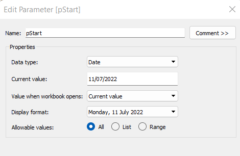
pStart
Date parameter defaulted to 11/07/2022 (11th July 2022), with a display format of <weekday>, <date>
pEnd
As above, but defaulted to 24/07/2022 (24th July 2022).
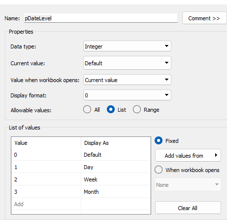
pDateLevel
integer with values 0-3 as listed below, with a text Display As. Defaulted to ‘Default’. Note, I am using integers as we will be referencing them in IF statements later, and integers are more performant than comparing strings.
With these parameters, we can then build
Date To Display
DATE( IF [pDateLevel] = 0 THEN IF DATEDIFF(‘day’, [pStart], [pEnd]) < 28 THEN DATETRUNC(‘day’,[Date]) ELSEIF DATEDIFF(‘day’, [pStart], [pEnd]) < 90 THEN DATETRUNC(‘week’, [Date]) ELSE DATETRUNC(‘month’, [Date]) END ELSEIF [pDateLevel] = 1 THEN DATETRUNC(‘day’,[Date]) ELSEIF [pDateLevel] = 2 THEN DATETRUNC(‘week’,[Date]) ELSE DATETRUNC(‘month’, [Date]) END )
If the pDateLevel is set to 0 (ie Default), then compare the difference between the dates entered and truncate to the ‘day’ level if the difference is less than 28 days, the ‘week’ level if the difference is less than 90 days, else truncate to the month level (which will return 1st of the month). Otherwise, if the pDateLevel is 1 (ie Day), truncate to the day level, if it’s 2 (ie Week), truncate to the week level, else use the month level.
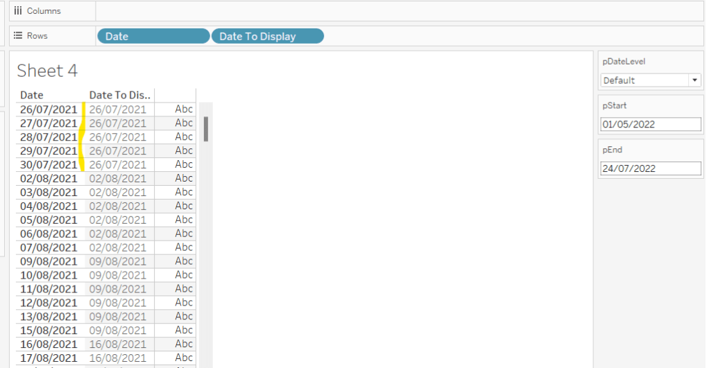
To see how this field is working, add Date and Date To Display to Rows, both as discrete exact dates (blue pills), display the parameter fields, and adjust the values. Below you can see that using the Default level, between 1st May and 24th July, the 1st day of the associated week against each date is displayed.
Building the Bar Chart
This is the simpler of the two charts to build, so we’ll start with this.
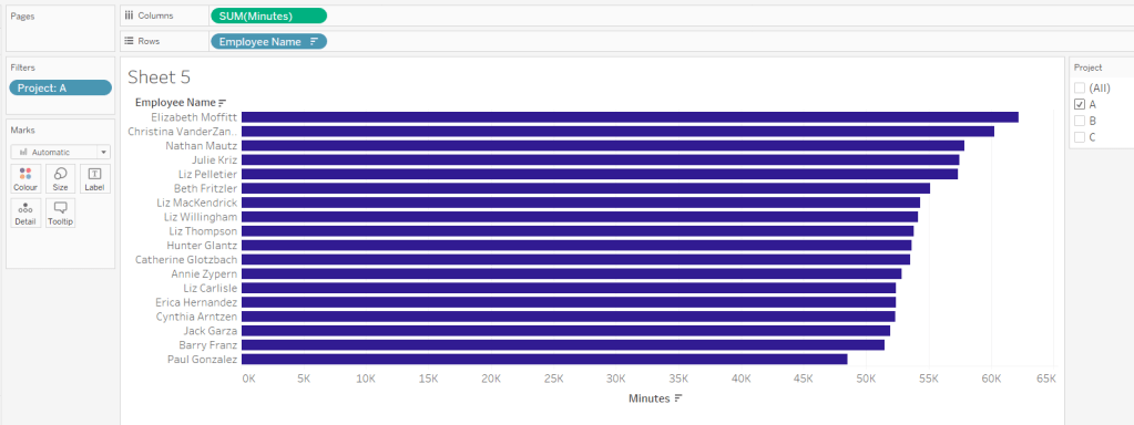
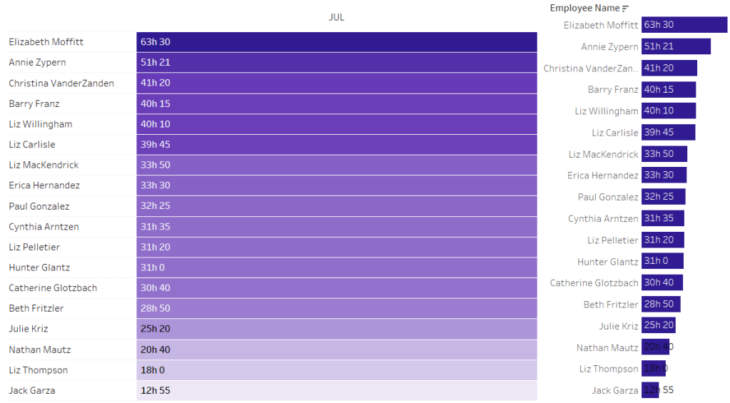
Add Employee Name to Rows, and Minutes to Columns. and sort by Minutes descending (just click the sort descending button in the toolbar). Add Project to Filter, select ‘A’ and then show the filter. Adjust the colour of the bars. I used #311b92
We need to restrict the data displayed based on the date range defined.
Dates to Include
[Date]>=[pStart] AND [Date]<=[pEnd]
Add this to the Filter shelf and set to True.
Now, we need to label the bars, and need new fields for this.
Duration (hrs)
FLOOR(SUM([Minutes])/60)
Using the FLOOR function means the value is always rounded down to the relevant whole number (eg 60.5 and above will still result in 60).
Format this field to be 0 decimal places with a ‘h’ suffix
Duration (mins)
SUM([Minutes])%60
Modulo (%) 60 means return the remainder when divided by 60. Format this to be 0 dp.
Add both these fields to the Label shelf, and adjust so the labels are displaying on the same line and are aligned to the left. You may need to increase the width of each row to see them.
Add Project to the Tooltip shelf and update, then remove all gridlines and the axis. Leave the Employee Name column visible for now. We’ll come back to this later.
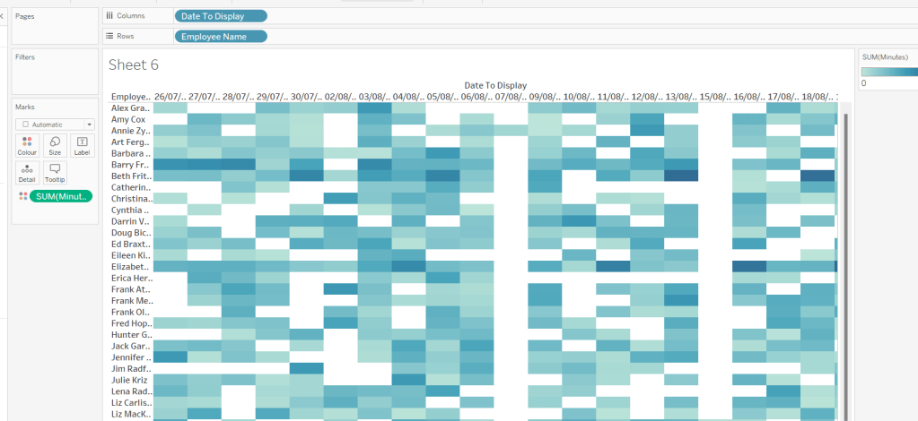
Building the Heat Map
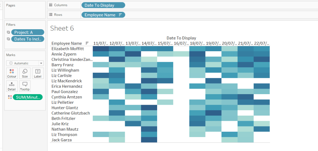
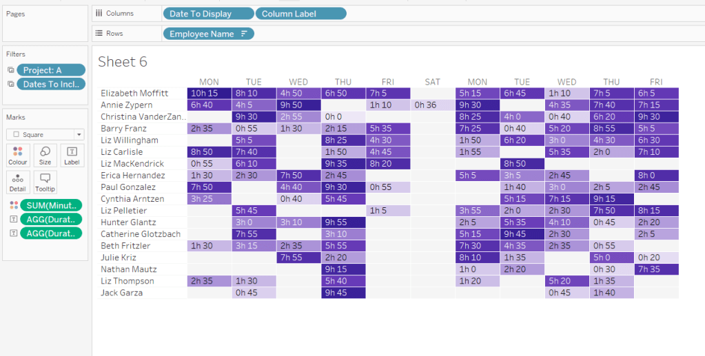
On a new sheet, add Employee Name to Rows and Date to Display as a discrete exact date (blue pill) to Columns. Add Minutes to Colour and a heat map should automatically display.
Go back to the bar sheet, and set both the Project and the Dates To Include filters to apply to the heat map worksheet as well (right click each pill on the filter shelf -> Apply to Worksheets -> Selected Worksheets and select the other one you’re building).
Then click the sort descending button in the toolbar, to order the data as per the bar.
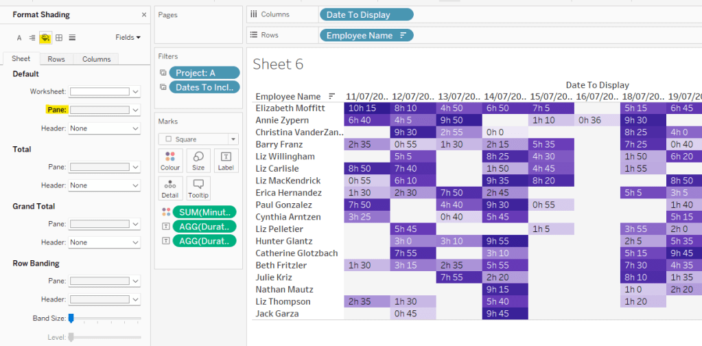
Add both Duration (hrs) and Duration (mins) to the Label shelf and change the mark type to Square. Adjust the label so it is on the same line and left aligned (I added a couple of spaces to the front of the text so it isn’t so squashed).
Edit the colours of the heat map – I used a colour palette I had installed called Material Design Deep Purple Seq which seemed to match, but may not be installed by default.
Format the main heat map section to have a light grey background by right clicking on the table -> format and setting the shading of the pane only to pale grey
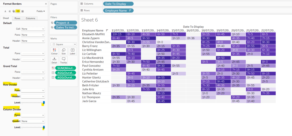
Then adjust the row dividers of the pane to be white, and the header to be pale grey (set the level to the max).
Adjust the column dividers similarly, setting the pane to be white, the header to none, and level to max
Next we want to deal with the column labels. By default they’re showing the date, but we want this to show something different depending on the date level being displayed.
Column Label
IF (([pDateLevel] = 1) OR (([pDateLevel] = 0) AND (DATEDIFF(‘day’, [pStart],[pEnd])<28))) THEN UPPER(LEFT([Weekday],3)) ELSEIF (([pDateLevel] = 2) OR (([pDateLevel] = 0) AND (DATEDIFF(‘day’, [pStart],[pEnd])<90))) THEN ‘w/c ‘ + IIF(LEN(STR(DATEPART(‘day’, [Date To Display])))=1,’0’+STR(DATEPART(‘day’, [Date To Display])), STR(DATEPART(‘day’, [Date To Display]))) + ‘-‘ + UPPER(LEFT(DATENAME(‘month’, [Date To Display]),3)) ELSE UPPER(LEFT(DATENAME(‘month’, [Date To Display]),3)) END
If the date level is ‘day’ or the date level is the default and the start & end are less than 28 days apart, then show the day of the week (1st 3 letters only in upper case).
Else if the date level is ‘week’ or the date level is the default and the start & end are less than 90 days apart, then show the text ‘w/c’ along with the day number (which should be 01 to 09 if the day is < 10) a dash (-) and then the 1st 3 letters of the month in upper case.
Else, we’re in monthly mode, so show the 1st 3 letters of the month in upper case.
Add this to the Columns shelf, then hide the Date To Display field (uncheck show header), hide field label for columns and hide field label for rows. Format the Employee Name field so its a different font (I changed to Tableau Book).
Again play around with the parameters and see the changes to the column label.
Finally, add Project to the Tooltip and update. You’ll need to adjust the formatting of the Date To Display field to get it into <day of week>, <date> format.
Adding to the Dashboard
When you add the two charts to the dashboard, you’ll need to set them side by side within a horizontal layout container. Remove the titles. They both need to be set to ‘fit entire view’, and the width of the heat map chart should be fixed (I set it to 870px), so it retains the space it stays in, even when you only have 1 month displayed.
Once you’re happy the order of the heat map employees matches the order of your bar chart, uncheck show header against the Employee Name field on the bar chart.
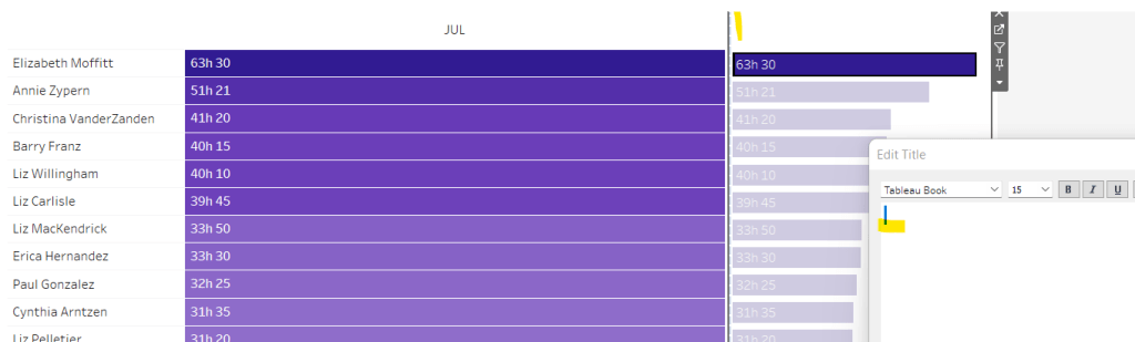
To get the bars to align with the heat map, I showed the title of the bar, removed the text and just entered a space. This dropped the bars so they just about aligned. You may need to tweak by increasing the size of the bars slightly.
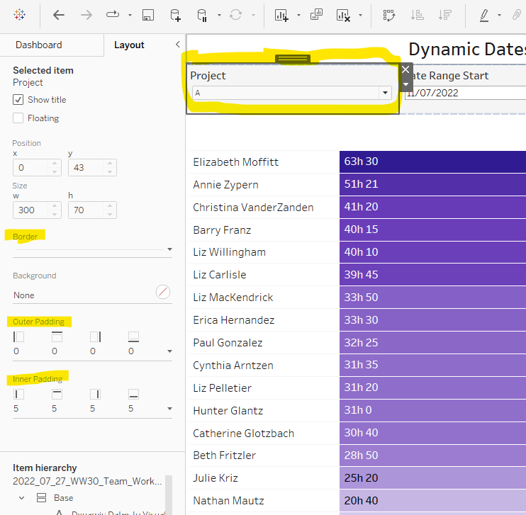
Finally, you need to move your parameters around. I placed them in a horizontal container, whose background colour was set to pale grey. I then set the objects within to be equally spaced by setting the container to Distribute Contents Evenly.
I then altered the padding of each of the parameter objects to have outer padding = 0 and inner padding = 5 and added a pale grey border surrounding each.
With #TC21 looming next week, Candra’s set this week’s challenge, based on inspiration from past Tableau Conferences – a simple looking, but effective visualisation for understanding profit performance within some pre-established timeframes.
Building the BANs
Identifying Top 5 / Bottom 5 / Everything Else
Building the Chart and Labelling the Bars
Adding the interactivity
Building the BANs
The timeframes we need to report over need to be based on a specific date. In this case it’s the latest date in the data set. If you were using this for a business dashboard, you might be basing it on Today / 1st of the Current Month etc. Rather than hardcode the date I need, I’ve worked out the latest month I want to use by
Set all the Order Dates in the data set to be the 1st of the month, then get the maximum of these dates. So as the last date in the data set is 30th Dec 2021, that’s been truncated to 1st Dec 2021 which is then what this field stores.
I then want to capture the profit values for each month, quarter, year into separate fields, so we have
Month
IF DATETRUNC(‘month’, [Order Date])=[Max Month] THEN [Profit] END
This only stores Profit values for rows where the Order Date is also in December
Quarter
IF DATETRUNC(‘quarter’,[Order Date])=DATETRUNC(‘quarter’,[Max Month]) THEN [Profit] END
This only stores Profit values for rows where the Order Date is in the same quarter as December (ie the 4th quarter which is months Oct-Dec).
Year
IF DATETRUNC(‘year’,[Order Date])=DATETRUNC(‘year’,[Max Month]) THEN [Profit] END
This stores Profit data for rows where the Order Date is in the same year.
All these fields are formatted to be $ with 0 dp.
A basic viz can the be built with Measure Names on Columns and Measure Names and Measure Values on Text. The Measure Names heading is then hidden, and the font and table formatting adjusted so the sheet looks as below.
Note – Naming these fields Month, Quarter, Year rather than Monthly Sales, Quarterly Sales etc, makes this display much easier and also helps with the interaction later.
Identifying the Top 5 / Bottom 5 / Everything Else
We need to be able to identify the Sub-Categories which have the best profits, those that have the worst, and the ‘rest’. We’re going to use Sets to help us with this. However the set entries could change depending on whether we’re looking by month, by quarter or by year. So first we need to create a field that is going to store the particular Profit value we need depending on what time period is being selected.
We need a parameter pDatePart to capture the time frame. This is a string field which is just defaulted to the text ‘Month’.
The interactivity later will set this parameter to the different values.
So now we know the ‘selected’ date part, we need to get the appropriate profit value
Value To Plot
CASE [pDatePart] WHEN ‘Month’ THEN [Month] WHEN ‘Quarter’ THEN [Quarter] ELSE [Year] END
This just uses the values from the 3 measures we created to start with.
So now we can create the sets we need. Right click on Sub-Category > Create > Set and create a set called Top 5 that is based on the Top 5 Value to Plot values
Then create another set in the same way called Bottom 5
With these sets, we can now determine the Sub-Category ‘label’ that will be displayed
Sub-Category Display
IF [Top 5] OR [Bottom 5] THEN [Sub-Category] ELSE ‘Everyone Else’ END
and the grouping that will be used to colour the bars
Sub Cat Group
IF [Top 5] THEN ‘Top 5’ ELSEIF [Bottom 5] THEN ‘Bottom 5’ ELSE ‘Everything Else’ END
Building the Chart & Labelling the Bars
Ok, so now we’ve got the building blocks in place, we can build the chart. You will probably be tempted to build a bar chart (I did to start with), but positioning the labels then became a bit tricksy. When we get to the labels, we’re going to need to use the left and right alignment options. However, when you build a bar chart, if you right align the label, the label will be positioned outside at the end of the bar (even though this seems a little odd with negative values, as it looks to be on the left…).
Right aligned labels
But then we set the labels to be left aligned, the labels appear inside the bar instead, and not outside on the left.
Left aligned labels
So instead, rather than using the bar mark type, we need to build this chart using the gantt mark type, and base the Size on the Value to Plot field.
However, the value being plotted is actually an average value based on the number of Sub-Categories being ‘grouped’ as otherwise the value associated to Everything Else can end up bigger than all the rest. I created the following field
Avg Value To Plot
SUM([Value to Plot])/COUNTD([Sub-Category])
formatted to $ with 0dp.
So now we start building by adding Sub-Category Display to Rows and type in MIN(0) into Columns. Change the mark type to Gantt and add Avg Value To Plot to Size. Add Sub-Cat Group to Colour and adjust accordingly. Sort the Sub-Category Display field by Avg Value To Plot descending.
Now we can’t just label by a single field of the value or the sub-category, as while the ‘automatic’ label alignment option, almost puts the labels in the right positions, there is no way to define an ‘opposite’ to the ‘automatic’ alignment. We need to define some dedicated label fields based on where we want them to display.
Label – Left – Profit
IF [Avg Value To Plot]<0 THEN [Avg Value To Plot] END
If we’re in the bottom half of the chart, we’re going to display the Profit value on the left side.
Label – Left – Sub Cat
IF [Avg Value To Plot]>=0 THEN ATTR([Sub-Category Display]) END
If we’re in the top half of the chart, we’re going to display the Sub-Category Display on the left side.
Add both these fields to the Label shelf and then adjust the label alignment to be left.
To label the other ends, we need to create two further label fields
Label – Right – Profit
IF [Avg Value To Plot]>=0 THEN [Avg Value To Plot] END
Label – Right – Sub Cat
IF [Avg Value To Plot]<0 THEN ATTR([Sub-Category Display]) END
We then need to create another MIN(0) on Columns (easiest way is to hold down control, then click on the existing MIN(0) field and drag it next to itself to create a duplicate. Then on the 2nd marks card, remove the two Label – Left – xxx fields and add the two Label – Right -xxx fields. Change the alignment to right.
The make the chart Dual Axis and synchronise the axis.
Now you can hide the Sub-Category Display header from showing, hide the axis, remove gridlines etc.
Adding the interactivity
Once the two sheets are on the dashboard, you can add a dashboard parameter action which will on select of the KPI/BAN chart, pass the Measure Name into the pDatePart parameter. When the mark is unselected, the parameter value should stay as it is.
And hopefully, you should now have a working viz. My published version is here.
This week’s #WOW challenge was a joint one with the #PreppinData crew, with the intention to use the #PreppinData challenge to create the data set needed for the Tableau challenge. I completed the Prep challenge, but decided to use the output provided by the #PreppinData crew as the input to this challenge (just in case I had inadvertently ended up with discrepancies).
Sport Selector
Adjusting the time
The Schedule Viz
Event Counts in Tooltip
Event listing Viz in Tooltip
Other Sports bar chart Viz in Tooltip
Dashboard interactivity
Sport Selector
This is a simple chart that lists the Sport Groups. I chose to build a bar chart using MIN(1) on the Columns and Sport Group on Rows. The axis was then fixed from 0-1.
Create a set based on Sport Group and select a few values to be ‘in’ the set (eg Boxing, Gymnastics, Martial Arts).
Add the Sport Group Set to the Colour shelf to identify the selected sports. Adjust colours accordingly.
Adjusting the Time
Create a parameter pTimeAdjust which is an integer paramater, defaulted to 0 and ranges from -12 to +12. Set the step value to 1 as this will ensure when you add the parameter to the dashboard, the prev/next buttons can be displayed alongside the slider.
Create a calculated field to store the time of the event based on the ‘timezone’ selected via the above parameter
Date Time Adjust
DATEADD(‘hour’, [pTimeAdjust], [UK Date Time])
This field will be used to display the full event date & time on the event listing viz in tooltip, along with building the schedule viz itself.
Additionally, create a field based on the above, which just stores the day of the adjusted datetime field above
Day of Adjusted Date
DATE(DATETRUNC(‘day’,[Date Time Adjust]))
This field is needed to help with the filtering required for the viz in tooltips to display.
The Schedule Viz
Add Date Time Adjust set to the Month datepart (blue pill) to the Columns shelf, and alongside it add the same field set to the Day datepart (blue pill). On the Rows, add Sport Group and Sport. Add the Sport Group Set to the Filter shelf. This will give you the ‘bones’ of the schedule
In viewing the provided solution, there was a bit of a discrepancy between when a ‘medal’ icon should show or not, compared to the Medal Ceremony? field provided in the data. It transpired Lorna had made an adjustment, as there were some events that had a ‘final’, but did not include a gold medal or ceremony event.
So to try to match up with Lorna’s output, I too made adjustments, but I can’t guarantee it matches any published solution.
First up I identify the Victory Ceremony events
Is Victory Ceremony?
CONTAINS([Event],’Victory Ceremony’)
I chose to exclude all these events from the schedule, so this field is added to the Filter shelf and set to False.
I also identify the events which appear to be a ‘final’
Is Final?
CONTAINS([Event],’Gold Medal’) OR CONTAINS([Event],’ Final’)
This field will separate the events into two types. Change the MarkType to Shape, then add this field onto that shelf. Set the shapes accordingly. Note – to add the medal shape, save the image Lorna provided to your machine, then follow these instructions so it’s available for selection.
I chose to add the Is Final? to the Size shelf too, so the shapes can be adjusted to something more suitable.
If you add the rows and columns dividers, you’ll notice the single circles aren’t centred. To resolve this, we’re going to need some axis.
Add MIN(1) to the Rows shelf (y-axis). This will give us some vertical headspace.
Now we need to manage the horizontal space, and ensure the marks don’t overlap each other. When there’s no finals, we want the circle to be plotted in the middle. When there’s both non-final and final ‘events’ we want the two marks to be off-centre, one to the left and one to the right.
We need some calculations to help with this.
#Events by Sport Per Day
{FIXED [Day of Adjusted Date], [Is Victory Ceremony?],[Sport]: COUNT([Event Schedule])}
This helps us count the number of of events per day for a specific sport
#Event Finals By Sport By Day
{FIXED [Day of Adjusted Date], [Is Victory Ceremony?],[Sport]: SUM(IIF([Is Final?],1,0))}
This basically helps us count the number of finals for each sport on a day.
With this we can build
X-Axis
IF [#Event Finals by Sport Per Day] =0 THEN 5 ELSEIF [#Event Finals by Sport Per Day]-[#Events by Sport Per Day] =0 THEN 5 ELSEIF [Is Final?] THEN 7 ELSE 3 END
If there’s no final, plot at 5, if there’s only a final, plot at 5 otherwise plot a final at 7 and a non-final at 3.
Add this to the Columns shelf (set to be a dimension ie not SUM), and edit the axis to be fixed from 0-10.
Events Count in Tooltip
I was also a bit puzzled by some of the numbers being displayed in the tooltip, so chose to compute and show the following 3 measures
Number of Events for Sport on that day (this is the #Events by Sport per Day already calculated)
Number of Event Finals for Sport on that day (this is the #Event Finals by Sport by Day already calculated)
Total Number of events for all other sports on that day (ie the selected sport is excluded from the count).
SUM([# Events Per Day]) – SUM([#Events by Sport Per Day])
Pop all these on the Tooltip shelf and format appropriately.
You’ll also need to add the Day of Adjusted Date to the Tooltip. This should be set to exact date and discrete (blue pill).
Event Listing in Tooltip
Build out a data listing view of Sport Group, Sport, Date Time Adjust and add Event (I renamed the Event Split field) to the Text shelf. Add Day of Adjusted Date to the Detail shelf. Hide Sport Group and format.
On the schedule viz, add this worksheet to the tooltip, passing Sport and Day of Adjusted Date as filters on the string
Other Sports bar chart Viz in Tooltip
Once again this is a relatively simple chart to build out, with the Day of Adjusted Date field hidden in the display (but necessary for the VIT to filter properly).
However, this will display all sports, and we need this chart to not show the sport that has been initially selected (hovered).
Create a parameter pSportToExclude which is a string parameter. For the purpose of demonstration, enter the text Football.
Create a field
Excluded Sport?
[Sport]=[pSportToExclude]
Add this field to the Filter shelf and set to False, and the sport will disappear from the list
Add a reference to this sheet from the tooltip of the schedule viz, this time passing just Day of Adjusted Date as the filter.
Dashboard Interactivity
Hide / Show Sport Selector
When adding the Sport Selector sheet and the Schedule viz to the dashboard, you need to make sure they exist side by side in the same horizontal container.
Then, providing you are using v2021.2, you can set the Sport Selector object to Hide/Show. See this video for help.
Add remove sports
You will need 2 dashboard set actions for this. They should run on ‘menu’, and one will add items to the set, and the other remove
Set the selected sport to exclude
We’ll use a parameter action for this to run on hover and set the pSportToExclude parameter
Stop Sport Selector highlighting
Create a new field Dummy containing the text “Dummy” and add this to the Detail shelf of the Sport Selector viz.
The add a highlight action against this sheet only
Hopefully I’ve ticked off all the core elements here. There was a fair bit going on, and I’m conscious I’ve drafted this blog fairly quickly in comparison. My published viz is here .
Note, there are a couple of elements in my viz that I added which weren’t on the original solution. I’ve chosen not to include in the blog as the images/characters I chose to use didn’t render on Tableau Public. If you download the workbook, you’ll be able to see what my intention was.
I did also create an alternative view ‘heatmap’ style view as well which you can see here.
Week 20 for #WOW2021, and Lorna Brown set the challenge based on comparing dates. The requirement was to avoid LoDs in preference of table calculations. Unintentionally, I managed to build a solution without table calcs either. This just happened based on the problem solving process I ended up taking. I figured I would encounter a need for a table calc as I progressed, but it didn’t happen.
Defining the key calculated fields
Building the BAN
Building the Line Chart
The Reset button
Adding the dashboard interactivity
Defining the key calculated fields
To drive this viz, you’ll need 2 parameters – one to store the selected date and one for the selected comparison timeframe.
pSelectedDate
pComparison
Set to be an integer (more efficient in calcs later), but display text on screen
We now need to work out what the comparison date will be for each of the selections.
We’ll start with the date last year. We’re looking for the ‘equivalent’ day of the year in the previous year. I didn’t read the hint provided, so came up with my own method based on the month and whether we’re in a leap year or not
Equivalent Day Last Year
DATE(IF ((DATEPART(‘month’,[pSelectedDate]) <=2) AND ((YEAR([pSelectedDate])-1)%4=0)) OR ((DATEPART(‘month’,[pSelectedDate])>=3) AND (YEAR([pSelectedDate])%4=0)) THEN DATEADD(‘day’,2,DATEADD(‘year’,-1,[pSelectedDate])) ELSE DATEADD(‘day’,1,DATEADD(‘year’,-1,[pSelectedDate])) END)
So what is this saying….
If the month of the pSelectedDate is Jan or Feb AND the previous year is a leap year (as it can be divided by 4 with no remainder), OR if the month of pSelectedDate is not Jan or Feb and this year is a leap year, then get the exact same date from last year, but add on 2 days, otherwise get the exact same date from last year, but add on just 1 day.
Now let’s consider the same day for last month. I played with Lorna’s solution, entering difference dates to see what the compare date came back as, and it wasn’t always clear to me what the logic was that was being used. So this is what I came up with. If the pSelectedDate was for example, the 3rd Tuesday in the month, then I wanted to get the 3rd Tuesday in the previous month. However, based on the length of months and when months start and end, some months can have nearly 5 weeks in a month, while the previous may only have 4. In my logic therefore, if there was no 5th Tuesday in the previous month, I would return the 4th Tuesday of the month. So in that instance if pSelectedDate is the 4th Tuesday in the month, I’d compare to the 4th Tuesday of the previous month. If pSelectedDate is moved to the 5th Tuesday in the same month, it would also compare to the 4th Tuesday of the previous month – PHEW! all a bit mind boggling perhaps, and it certainly took the most amount of time in this challenge.
I broke this down into multiple calculations.
DoW Selected Date
DATEPART(‘weekday’,[pSelectedDate],’Sunday’)
What is the day of the week number for the pSelectedDate? If pSelectedDate is 18th May 2021, this will be 3 (ie Tuesday).
Exact Date Prev Month
DATE(DATEADD(‘month’, -1, [pSelectedDate]))
as it says on the tin – exact same date last month, so if pSelectedDate is 18th May, this will be 18th April.
Prior DoW Prev Mth
DATE(CASE [DoW Selected Date] WHEN 1 THEN DATETRUNC(‘week’, [Exact Date Prev Month],’Sunday’) WHEN 2 THEN DATETRUNC(‘week’, [Exact Date Prev Month],’Monday’) WHEN 3 THEN DATETRUNC(‘week’, [Exact Date Prev Month],’Tuesday’) WHEN 4 THEN DATETRUNC(‘week’, [Exact Date Prev Month],’Wednesday’) WHEN 5 THEN DATETRUNC(‘week’, [Exact Date Prev Month],’Thursday’) WHEN 6 THEN DATETRUNC(‘week’, [Exact Date Prev Month],’Friday’) WHEN 7 THEN DATETRUNC(‘week’, [Exact Date Prev Month],’Saturday’) END)
If pSelectedDate is a Tuesday, then this returns the date of the Tuesday that is before the exact date last month. If pSelectedDate is Tuesday 18th May, Exact Date Prev Month is 18th April, which is a Sunday. Truncating this date to the start of the week, where the week starts on a Tuesday, returns Tues 13th April.
Next DoW Prev Mth
DATE(DATEADD(‘week’, 1, [Prior DoW Prev Mth]))
Just adds 1 week onto the above.
Equivalent Day Last Mth
IF MONTH([pSelectedDate]) = MONTH([Next DoW Prev Month]) THEN [Prior DoW Prev Mth] ELSE [Next DoW Prev Month] END
If the months of pSelectedDate and New DoW Prev Mth are the same, then use the ‘previous’ date, otherwise use the ‘next date’. This took some pen and paper to work out!
So now having worked out what the dates might be, I just plugged them into the below to get the comparison date we need.
Compare Date
DATE(IF [pComparison] = 1 THEN [Equivalent Day Last Year] ELSEIF [pComparison] = 2 THEN [Equivalent Day Last Month] ELSE DATEADD(‘week’, -1, [pSelectedDate]) END)
Further fields we then need are
Selected Date Sales
IF [Order Date] = [pSelectedDate] THEN [Sales] END
Compared Date Sales
IF [Order Date] = [Compare Date] THEN [Sales] END
% Difference
(SUM([Selected Date Sales]) – SUM([Compared Date Sales])) / SUM([Compared Date Sales])
custom formatted to ▲0.0%;▼0.0%
Building the BAN
I built this using a bar mark type with MIN(1) on Columns and the axis fixed from 0 to 1.
Then all the relevant fields were added to the Label field and organised accordingly. All date fields were formatted to the <weekday>, dd mmmm, yyyy format.
The % Difference field was added to Colour, and then the colour legend formatted as below
Building the Line Chart
The line chart only needs to show the information between the Compare Date and the pSelectedDate.
Dates to Show
[Order Date]>=[Compare Date] AND [Order Date]<=[pSelectedDate]
This needs to be on Filter shelf and set to True.
The main line chart is then just simply Order Date (exact date, continuous) plotted against Sales
For the circle markers, we can add Selected Date Sales and Compared Date Sales as ‘shared measures’ onto another axis
To get the ‘label’ points to show, we’re going to plot 2 more marks at an arbitrary point on the axis, but at the dates we care about. For this I created
Minus 500
IF [Order Date] = [pSelectedDate] OR [Order Date]= [Compare Date] THEN -500 END
Add this into the MeasureValues section, but aggregated to Avg rather than Sum
We want to label these marks, but not with the -500 value.
Selected | Compared Date Sales
IF [Order Date] = [pSelectedDate] THEN ([Selected Date Sales]) ELSEIF [Order Date] = [Compare Date] THEN ([Compared Date Sales]) END
Add this field onto the Label shelf of the Measure Values marks card and show mark labels
But we only want the labels to show against the lower marks. I have to admit I tried many things to try to make this work, but in the end had to peek at Lorna’s solution. The label setting needs to be – its the Measure Names field that is key here!
I then set the colour of the Minus 500 measure to white, so you can’t see it
This chart can then be set to dual axis (don’t forget to synchronise those axis). You may need to reset some of the mark types etc. Remove all headers/borders/gridlines.
The Reset Button
I created a Default Date field storing DATE(#2021-05-18#) and added to a sheet as below.
Adding the dashboard interactivity
On click of a point on the chart, it should set the pSelectedDate parameter. This is a parameter action.
We don’t what the chart to show the point as ‘selected’/highlighted though, so we need to use a dashboard filter action to supress this from happening.
Create fields True = True and False = False. Add these 2 fields to the Detail shelf on the line chart.
Then on the dashboard, add a dashboard filter action as below, setting the fields to map True to False.
Finally, the reset button needs to set the parameter too :
Hopefully this should be enough to help you complete this challenge. My published viz is here.
Once again, I found this week tough! I understand the concept of parameter actions, and can use them for the ‘basics’, but the funky stuff people come up with to bend them to their will, is really beyond me.
I started the challenge with good intentions as always, ‘relating’ the Dates data to the Superstore data set matching the Date field to the Order Date field, built out the calendar view, but got stuck trying to figure out how to set the parameter action into an ‘End Date’ parameter, when I was already setting a ‘Start Date’ parameter. After staring at the screen for some time, I figured I’d try to work it all out from Ludovic’s viz instead.
There’s A LOT going on in this challenge, so I’ll do my best to explain.
Building the Calendar Picker
Building the Next / Previous control
Building the Year/Month control
Building the KPI & Trend Chart
Building the Calendar Picker
The calendar will only show 1 month, so let’s deal with that to start with.
A parameter will be used to store a date related to the month to show.
pMonthSelected
This is a date parameter that I chose to default to 01 June 2019.
Month Date
DATE(DATETRUNC(‘month’,[Date]))
This is truncating every Date in the dataset to the 1st of the relevant month
Month To Show
[pMonthSelected] = [Month Date]
Add this to the Filter shelf and set to True will limit the data to a single month, June 2019 by default.
To display the days of the month in the ‘grid’ layout, we need to know the day of the week each day falls on (so we know what column to position the day in), and we need to know what week in the year the day falls in, as this will dictate which row to position the day in.
Day of Week (Abbrev)
LEFT(DATENAME(‘weekday’, [Date]),3)
The basic calendar layout can then be built by
Month To Show = True on Filter
Day of Week (Abbrev) on Columns
WEEK(Date) on Rows
DAY(Date) on Text
The WEEK(Date) field is then hidden.
We’re going to need to represent each day by a ‘square’ block. I achieve this by adding MIN(1) to Columns, changing the mark type to Bar, fixing the axis from 0-1, then hiding the axis.
So now the basic calendar layout is achieved, we need to figure out how to select a start & end, and colour accordingly.
We’re going to use a single string parameter to store both the selected start & end dates, using a | to act as a delimiter allowing us to identify & so separate the 2 dates.
pSelectedDates
String parameter set to empty string by default
Show the parameter on the viz, and I will attempt to walk through the steps, showing how the values in the parameter influence other fields and what is displayed on the viz.
We need another field, that is going to be used in conjunction with the parameter. I’m going to build up what this field needs to store as we go through, so hoping it will all make sense.
Date Control
IF [pSelectedDates]=”” THEN STR([Date]) END
If the parameter is empty, then set Date Control to be the date.
Let’s add this to the Text so you can see what happens to this field.
So the first action we expect the user to take is to click on a single date displayed. This value stored in the Date Control field will be passed via the parameter action into the pSelectedDates field (I’ll show you how this works later). For now let’s assume the user has clicked on the 5th June, so type 2019-06-05 into the pSelectedDates field.
This is now the start date, and we need the Date Control field to change to reflect this
Date Control
IF [pSelectedDates]=”” THEN STR([Date]) ELSEIF [Date]<=DATE([pSelectedDates]) THEN STR([Date]) ELSE [pSelectedDates]+”|”+STR([Date]) END // else store start & end date
If the Date displayed is before that stored in the parameter, then Date Control will continue just to store the date, otherwise it will append | followed by the date onto the existing parameter value.
So when a date is clicked again, the value of the Date Control will once again be passed to the pSelectedDates parameter.
If the date clicked is earlier than the one already stored, eg let’s say 04 June was clicked, the Date Control value of 04 June is passed to the parameter, and is now the ‘start date’. Type 2019-06-04 into the pSelectedDates field.
But if a later date is selected, say 18th June, the Date Control value of 2019-06-04|2019-06-18 is passed into the pSelectedDates parameter, and we now need another step with our Date Control field :
Date Control
IF [pSelectedDates]=”” THEN STR([Date]) ELSEIF CONTAINS([pSelectedDates],”|”) THEN STR([Date]) ELSEIF [Date]<=DATE([pSelectedDates]) THEN STR([Date]) ELSE [pSelectedDates]+”|”+STR([Date]) END
The 2nd statement is now looking for the | character and if it finds it, we know a start & end dates has been selected, so we need to ‘reset’ this control field to how it was originally – just it’s own date.
Type in 2019-06-04|2019-06-18 into the pSelectedDates field to see this.
Ok, so now we can see how the pSelectedDates field is working with the Date Control field, we now need to define some additional fields to help us identify the start & end of the dates selected, so we can work out what to colour.
This is looking for the position of the | field and taking everything from the first character in the pSelectedDates string up to the character before the |.
NoteI originally used DATE(SPLIT([pSelectedDates], “|”,1)), but after extracting the data set, this calculation caused errors. I don’t know why, but the above workaround sufficed.
Find the position of the | and take all the characters starting at the position after the | and ending at the character 10 characters later (the date format is 10 characters so this can be easily hardcoded)
COLOUR: Date
IF [Date]= [Date Selection Start] OR [Date] = [Date Selection End] THEN ‘Hot Pink’ ELSEIF [Date] > [Date Selection Start] AND [Date] < [Date Selection End] THEN ‘Pink’ ELSE ‘White’ END
Add this onto the Colour shelf, and adjust accordingly
We can remove the Date Control from Text now, but it needs to remain in the view, so it can be referenced when we build the parameter action. Add it onto Detail shelf instead.
Finally add this viz onto a dashboard, then add the parameter action, setting the Target Parameter to pSelectedDates and the Field to pass as Date Control.
As you play around selecting values on the dashboard, you’ll notice the dates appear ‘greyed out’, as the ‘on click’ action is essentially highlighting what you’ve selected. To stop this from happening create a calculated field called True that just stores the value of True and and a calculated field called False that stores the value False. Add both of these to the Detail shelf of the calendar viz.
Then on the dashboard, add a Filter action that goes from the dashboard to the sheet itself, passing the values Source: True = Target: False
Building the Next / Previous Control
We need to store the value of the next month related to the Date unless we’re already in the last month of the data set, in which case we’ll just keep the same month (ie if the month is 01 Nov 2019, next month will be 01 Dec 2019, but if the month is 01 Dec 2019 which is the last month in the data set, the next month will also be 01 Dec 2019. This stops the next control from moving forward when we reach the end.
Next Month
IF [Month Date] = {MAX([Month Date])} THEN [Month Date] ELSE DATE(DATEADD(‘month’, 1, [Month Date])) END
Change the mark type to Shape and select an appropriate arrow. If need be reduce the transparency of the shape colour (I chose 50% which changed a black arrow to look like a grey arrow).
On a new sheet, Add Month To Show = True to the Filter shelf, and Next Month to the Detail shelf.
If you recall, right at the start, we created a pMonthSelected parameter, and this will be used to change the month displayed.
Add the viz to the dashboard, and add a parameter action that on select, targets the pMonthSelected parameter, passing in the Next Month field
For the Previous Month control, we need apply similar steps, but using the field below instead.
Prev Month
IF [Month Date] = {MIN([Month Date])} THEN [Month Date] ELSE DATE(DATEADD(‘month’, -1, [Month Date])) End
Building the Year/Month control
When building the Year selector, we need to filter the data to just the month name already selected/in view, which is based on the pMonthSelected parameter. Ie if the month selected is 01 June 2019, we want the data related to June 2016, June 2017, June 2018, June 2019
Add this to the Filter shelf, set to true, then build out the view as below, fixing the axes between 0-1 again, and then hiding. You can see the values of the Month(Date)) displayed, and it’s this field that will be passed via a parameter action. It can be moved to Detail.
COLOUR:Selected Year
YEAR([pMonthSelected])=YEAR([Date])
Add this to the Colour shelf and adjust accordingly.
When added to the dashboard, the associated parameter action required is :
When building the month selector, we need a similar filter to ensure the months shown are all associated to a single year
Filter Year
YEAR([pMonthSelected]) = YEAR([Date])
Add this to the Filter shelf set to True.
The layout of the Months, requires some additional fields to determine which row and column the month should be positioned in.
Month Cols
IF (DATEPART(‘month’,[Date]) %4) =0 THEN 4 ELSE (DATEPART(‘month’,[Date]) %4) END
DATEPART returns the integer value of the month, ie a number between 1-12, so this calculation is using the modulo (%) function to position based on the remainder when dividing the month number by 4.
Month Row
IF DATEPART(‘month’,[Date]) <=4 THEN 1 ELSEIF DATEPART(‘month’,[Date]) <= 8 THEN 2 ELSE 3 END
Adding these to the view as follows gives us a grid
Note the blue Month(Date) on the Text shelf is showing just the month name ie ‘January’, and has been formatted to it’s abbreviation. The green Month(Date) on the Detail shelf is storing the full month year ie January 2019.
COLOUR:Selected Month
[pMonthSelected]=[Month Date]
Add to the colour shelf and adjust accordingly.
You can then hide the Month Col & Month Row fields from displaying.
When added to the dashboard, the associated parameter action required is
Note You will need to apply the same ‘true=false’ trick described earlier to both these views using filter actions to prevent them from highlighting on selection.
Hiding the year/month selector
On the dashboard add a vertical container, then place the Year Selector sheet and the Month Selector inside.
Remove the chart titles, set the background of the container to white, then set the container to be floating and select the container option to Add Show/Hide Button.
You’ll need to spend some time adjusting the size and the position of the floating container once you have the layout of all the other objects finalised.
Building the KPI & Trend Chart
I’m going to try to be brief with this section. The above is A LOT to take in and write!
Selected Period
This is simply using the Date Selection Start & Date Selection End fields to display in a text field
KPI BANs
We need to be able to filter the data being displayed based on the selection
Dates to Show
[Date]>= [Date Selection Start] AND [Date]<= [Date Selection End]
This is added to the Filter shelf and set to True.
After that we’re just building a simple Text based viz utilising Measure Names & Measure Values as shown below
And finally the trend chart, again needs to be filtered by Dates To Show = True, and is a simple line chart plotting Date against the measures required as below
When added to the dashboard, these 2 sheets should be placed side by side in a horizontal container, both set to fit entire view. The right padding should be set to 0 for the KPI chart and the left padding set to 0 for the trend chart. This will have the effect of the horizontal lines for each chart joining together to make it look like a single chart.
Phew! I’m beat! My published viz is here. Keeping fingers crossed for a challenge that is easier to blog about next week 🙂