For this week’s challenge, Kyle revisited a previous challenge from 2020, but remade it over utilising some of the newer features of Tableau, specifically Dynamic Zone Visibility. I blogged my solution to the original challenge here, so this blog will lift some of the techniques (and documentation) I employed directly.

Define the parameters

The first step in this challenge is to define all the parameters needed, these being :

pDateSelector

A string parameter just set to contain the value Last 30 Days

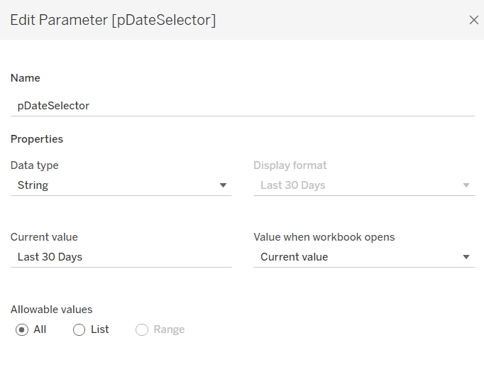
This parameter will be set via a Parameter Action, so there is no need to define this a list with all the options.

pDays

An integer parameter defaulted to 120

pStartDate

A date parameter defaulted to 01 Jan 2023

pEndDate

Another date parameter defaulted to 01 Aug 2023

The chart needs to adjust based on a measure selected, so we need to capture the measure option selected

pSelectedMeasure

string parameter defaulted to Sales

This parameter will be set by a parameter action, so again there is no need to actually list the possible values.

Finally, I also created a parameter

pToday

Date parameter defaulted to 02 May 2023.

The requirements indicate the information displayed should be restricted to ‘today’, using the TODAY() function. However given the data set is static, if I use TODAY() and look at this in a year’s time, nothing will show. So instead I have ‘hardcoded’ ‘today’ using this parameter.

Using this parameter I then created

Order Date < Today

[Order Date] <= [pToday]

and added this as a data source filter set to True. This ensures that all the sheets I build is then automatically ignoring and data where the Order Date is 3rd May 2023 onwards.

Building the time-series chart

We need to determine which measure to show based on the selection made by the user and stored in the pSelectedMeasure parameter. This will be Sales, Profit or a count of the number of orders. First we need to create

Count Orders

COUNTD([Order ID])

and then we can create

Measure to Display

CASE [pSelectedMeasure]
WHEN ‘Sales’ THEN SUM([Sales])
WHEN ‘Profit’ THEN SUM([Profit])
WHEN ‘Orders’ THEN [Count Orders]
END

Add Order Date set to the continuous day level (green pill) to Columns and Measure to Display to Rows. This gives us all data from the earliest day in the data set up to 2nd May 2023.

We need to restrict this based on the ‘date selector’, so create

In Timeframe

CASE [pDateSelector]
WHEN ‘Last 30 Days’ THEN [Order Date]>DATEADD(‘day’,-30,[pToday])
WHEN ‘Last N Days’ THEN [Order Date]>DATEADD(‘day’,-1*[pDays],[pToday])
ELSE [Order Date]>=[pStartDate] AND [Order Date]<=[pEndDate]
END

If ‘last 30 days’, get the data that is greater than 30 days ago; if ‘last n days’, get the data that is greater than the last ‘n’ days ago, otherwise get the data between the start & end dates specified.

Add this to the Filter shelf and set to True.

Add another instance of Measure to Display to Rows, make dual axis and synchronise axes. Change the mark type of the first marks card to be Area and set the other to explicitly be a line.

Add pSelectedMeasure to the Colour shelf of the All marks card. Adjust the colour of the ‘Sales’ value accordingly.

If you’re not already displaying it, show the pSelectedMeasure parameter input, and manually change the value by typing in ‘Profit’. The chart will change colour, so again adjust accordingly. Repeat the process by typing in ‘Orders’.

Set the parameter back to ‘Sales’.

The tooltip needs to display different formatted values, so we need a couple of fields to handle this

Tooltip- Sales or Profit

IF [pSelectedMeasure] <> ‘Orders’ THEN [Measure to Display] END

Format this to $ with 0 dp, and set to use ( ) when value is negative.

Tooltip – Orders

IF [pSelectedMeasure] = ‘Orders’ THEN [Measure to Display] END

Format this to a number with 0 dp.

Add both these fields to the Tooltip shelf of the All marks card, and adjust the tooltip accordingly, positioning the two ‘Tooltip’ fields directly adjacent to each other

Hide the right hand axis (right click, uncheck show header), and edit the left hand axis to set the axis title to be sourced from the pSelectedMeasure parameter

Remove all gridlines, zero line, axis ticks etc and row/column dividers, and edit the date axis to remove the axis title. Name the sheet ‘Chart’ or similar.

Building the BANs

1. Add Measure Names to Columns
2. Add Measure Names and Measure Values to the Text shelf
3. Add Measure Names to the Filter shelf and select just the 3 measures we’re interested in.
4. Reorder the columns to match the requirement

1. (Optional) Change the mark type to shape and set the shape to be a transparent shape (see this blog post for more details)
2. Change the formatting of the Measure Names and Measure Values on the Text shelf to set the size of the font to suit, and align middle, centre
3. Format the Sales and Profit measures to be $ with 0 dp and ( ) for neg values.
4. Add Measure Names to the Colour shelf and adjust colours to match the ones used on the line chart. (If you’ve used the transparent shape, edit the label to set the font to match mark colour).
5. Format the display to remove the row lines
6. Hide the Measure Names heading (right-click the Measure Names pill on the Columns shelf and unselect Show Header).
7. Add In Timeframe = True to the Filter shelf to restrict the data.
8. Uncheck the show tooltip option from the Tooltip shelf to stop the tooltip from displaying.
9. Name the sheet ‘BANs’ or similar

Building the Date Selector

On a new sheet, double click into the Columns shelf and type in MIN(0.0) Change the mark type to Shape.Create a new field

Label: Last 30 Days

‘Last 30 Days’

And add this to the Label shelf.

Create a new field

Is Selected Date Option – Last 30 Day

[pDateSelector] = [Label:Last 30 Days]

And add this to the Shape shelf. Adjust the shape for the ‘True’ value to be a filled circle.

Show the pDateSelector parameter and change the text in some way. This should change the ‘shape’ to ‘False’. Set this shape value to be an open circle.

Change the colour to be a dark grey, and increase the font size. Uncheck ‘Show Tooltip’.

Now type in another instance of MIN(0.0) to Columns. Create the following fields

Label:Last N Days

‘Last N Days’

and

Is Selected Date Option – Last N Days

[pDateSelector] = [Label:Last N Days]

ON the 2nd MIN(0.0) marks card, replace the fields on the shape and label shelves with these ones.

By default, the ‘last n days’ shape should be set to false, so make sure it’s an open circle. Change the value in the pDateSelector parameter to ‘Last N Days’ and the shape should now be ‘true’ – set to a closed circle.

Create a 3rd instance of MIN(0.0) on Columns and create

Label:Custom Dates

‘Custom Dates’

and

Is Selected Date Option – Custom Dates

[pDateSelector] = [Label:Custom Dates]

and repeat the process above

Edit the axis of each to be fixed from -0.2 to 2. This has the effect of ‘left aligning’ the marks.

Hide the axis, and remove the row & column dividers, all gridlines and zero lines and axis lines.

Add Measure Names to the Detail shelf of the All marks card. The right click on Measure Names in the left hand data pane and select Alias. In the dialog box that presents, alias the 3 MIN(0.0) fields as per the 3 date selector options.

This step is the key to enabling the parameter action that will be set up to pass the appropriate ‘value’ into the pDateSelector parameter

Finally format the background of the whole worksheet to be grey.

Controlling the visibility of the selections

On the dashboard, I used a vertical layout container to add my title, the BANs and the Chart. Between the title and BANs, I added a horizontal container. On the left side of that I added the Date Selector sheet. On the right I then had another vertical container which contained other containers to display the start & end data parameters. It took a bit of ‘twiddling’ to get everything where I wanted.

I added the pDays parameter as a floating object and positioned it below the Last N Days option. I used the control visibility using value option to set this to display based on the value of the Is Selected Date Option – Last N Days calculated field.

Similarly, for the date input fields, I had the section all within a single container, so I set the visibility at the container level, rather than the object level (although you could repeat the step against all the objects you need to hide individually). For the container, I used the control visibility using value option to set this to display based on the value of the Is Selected Date Option – Custom Dates calculated field.

Adding the interactivity

To change the timeframe displayed in the BANs and chart, create a dashboard parameter action

Set Date Selection

On select of the Date Selector sheet, target the pDateSelector parameter, passing though Measure Names. When the selection is cleared, reset to ‘Last 30 Days’.

To change the measure displayed in the chart, create a dashboard parameter action

Select Measure

On select of the BANs sheet, target the pSelectedMeasurew parameter, passing through Measure Names. When the selection is cleared, reset to ‘Sales’.

Prevent the BANs and Selected Date option from being selected/highlighted

By default, clicking on one of the BAN numbers, or selecting an option in the date selector, will leave the option chosen ‘highlighted’ or ‘selected’ while the other options are ‘faded out’. To

Create two calculated fields

True

TRUE

False

FALSE

Add both these fields to the Detail shelf of the BANs sheet and the All marks card on the Date Selector sheet.

Then on the dashboard, create a dashboard filter action

Deselect BANs

On select of the BANs sheet on the dashboard, target the BANs sheet directly, passing through selected fields where True = False. Show all Values when the selection is cleared.

Repeat the exact process for the Date Selector sheet, creating a dashboard filter action called Deselect Date Selector.

You should now have a complete dashboard. My published viz is here.

Happy vizzin’!

Donna